9. Metrics for time series
Traditional metrics like the Euclidean distance are not always well suited for time series. Imagine a person saying a word slowly and another person saying the same quickly, and both persons are recorded. The output will be two unequal-length time series. Since both persons pronounce the same word, we can expect a metric between these two time series to be (close to) zero.
Specific metrics for time series have been developed, the most well-known being the Dynamic Time Warping (DTW) metric. Several variants have then been proposed because of downsides with the original formulation.
Metrics for time series can be found in the pyts.metrics module.
9.1. Classic Dynamic Time Warping
Given two time series  and
and  ,
the cost matrix
,
the cost matrix  is defined as the cost for each pair of values:

where  is the cost function.
is typically the squared difference:
is the cost function.
is typically the squared difference:  .
.
A warping path is a sequence  such that:
- Value condition:

- Boundary condition:
 and
and 
- Monotonicity and step-size condition:

The cost associated with a warping path, denoted  , is the sum of
the elements of the cost matrix that belong to the warping path:
, is the sum of
the elements of the cost matrix that belong to the warping path:

The Dynamic Time Warping score is defined as the minimum of these costs among all the warping paths:

where  is the set of warping paths. This score can be computed using
the accumulated matrix, denoted as
is the set of warping paths. This score can be computed using
the accumulated matrix, denoted as  , defined as:


The last entry of the accumulated cost matrix is the Dynamic Time Warping score:

The Dynamic Time Warping metric has two main downsides:
- Complexity: Computational complexity is
 .
. - It does not obey the triangle inequality, which means that a brute search must be performed when using a k-nearest neighbors algorithm for instance.
Several variants have been developed to address both downsides. We will describe the variants that address the first issue since the variants addressing the other issue are works in progress.
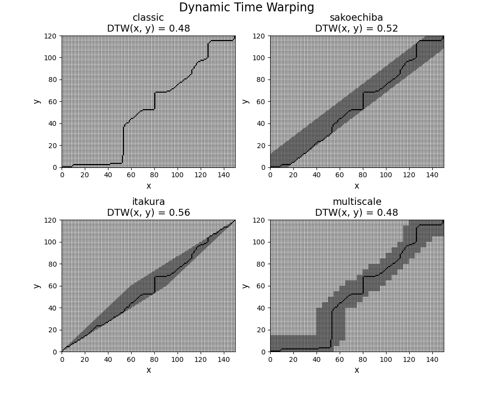
9.2. Variants of Dynamic Time Warping
The main idea is to reduce the set of warping paths in order to decrease the complexity of the algorithm. To do so, a region constraint is used. Two kinds of regions exist: global regions and adaptive regions.
9.2.1. Global regions
Global regions are regions that do not depend on the values of the time series
 and
and  , but only on their lengths.
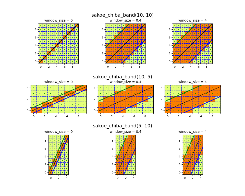
The most well-known global constraint region is the Sakoe-Chiba band and is
implemented as sakoe_chiba_band().
It is characterized by the window_size parameter.
Indices that belong to the band are indices that are not too far away from
the diagonal, that is:

where  is the
 window_size. The higher, the wider the region is.
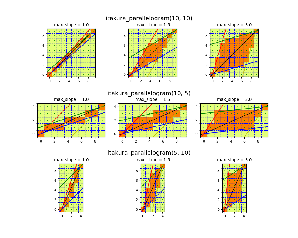
Another popular global constraint is the Itakura parallelogram and is
implemented as itakura_parallelogram().
It is characterized by the max_slope parameter, which defines how far away
two points can be.
The higher, the wider the region is.
9.2.2. Adaptive regions
Adaptive regions are regions that depend on the values of the time series
and . The idea is to find a constraint region that is more
specific to both time series.
One approach is called MultiscaleDTW. The idea is to down-sample both time series, so that they have fewer time points. The optimal path is computed for the down-sampled time series, then projected in the original space. This projection is the constraint region.
Another approach is called FastDTW. The idea is to repeat the process of down-sampling and defining the projected optimal path as the constraint region several times in a recursive fashion.
9.3. Implementations
The most convenient way to derive any Dynamic Time Warping score is to use
the dtw() function. dtw() has a method parameter that lets
you choose which variant to use (default is method='classic', which is
the classic DTW score). Options for each method can be provided with the
options parameter.
>>> from pyts.metrics import dtw
>>> x = [0, 1, 1]
>>> y = [2, 0, 1]
>>> dtw(x, y, method='sakoechiba', options={'window_size': 0.5})
2.0
References
- H. Sakoe and S. Chiba, “Dynamic programming algorithm optimization for spoken word recognition”. IEEE Transactions on Acoustics, Speech, and Signal Processing, 26(1), 43-49 (1978).
- F. Itakura, “Minimum prediction residual principle applied to speech recognition”. IEEE Transactions on Acoustics, Speech, and Signal Processing, 23(1), 67–72 (1975).
- M. Müller, H. Mattes and F. Kurth, “An efficient multiscale approach to audio synchronization”. International Conference on Music Information Retrieval, 6(1), 192-197 (2006).
- S. Salvador ans P. Chan, “FastDTW: Toward Accurate Dynamic Time Warping in Linear Time and Space”. KDD Workshop on Mining Temporal and Sequential Data, 70–80 (2004).
