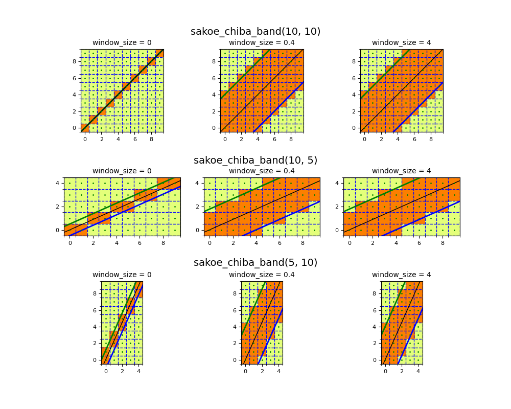
Sakoe-Chiba band

This example explains how to set the window_size parameter of the Sakoe-Chiba band when computing the Dynamic Time Warping (DTW) with method == "sakoechiba". The Sakoe-Chiba region is defined through a window_size parameter which determines the largest temporal shift allowed from the diagonal in the direction of the longest time series. It is implemented in pyts.metrics.sakoe_chiba_band(). The window size can be either set relatively to the length of the longest time series as a ratio between 0 and 1, or manually if an integer is given.

This example visualizes the Sakoe-Chiba band in different scenarios:

• the degenerate case: window_size = 0,
• a relative size: window_size = 0.4, and
• an absolute size: window_size = 4.

The last two cases are equivalent since 0.4 * 10 = 4.

# Author: Hicham Janati <hicham.janati@inria.fr>
#         Johann Faouzi <johann.faouzi@gmail.com>
# License: BSD-3-Clause

import numpy as np
import matplotlib.pyplot as plt

from pyts.metrics import sakoe_chiba_band
from pyts.metrics.dtw import _check_sakoe_chiba_params


# #####################################################################
# We write a function to visualize the sakoe-chiba band for different
# time series lengths.


def plot_sakoe_chiba(n_timestamps_1, n_timestamps_2, window_size=0.5, ax=None):
    """Plot the Sakoe-Chiba band."""
    region = sakoe_chiba_band(n_timestamps_1, n_timestamps_2, window_size)
    scale, horizontal_shift, vertical_shift = \
        _check_sakoe_chiba_params(n_timestamps_1, n_timestamps_2, window_size)
    mask = np.zeros((n_timestamps_2, n_timestamps_1))
    for i, (j, k) in enumerate(region.T):
        mask[j:k, i] = 1.

    plt.imshow(mask, origin='lower', cmap='Wistia', vmin=0, vmax=1)

    sz = max(n_timestamps_1, n_timestamps_2)
    x = np.arange(-1, sz + 1)
    lower_bound = scale * (x - horizontal_shift) - vertical_shift
    upper_bound = scale * (x + horizontal_shift) + vertical_shift
    plt.plot(x, lower_bound, 'b', lw=2)
    plt.plot(x, upper_bound, 'g', lw=2)
    diag = (n_timestamps_2 - 1) / (n_timestamps_1 - 1) * np.arange(-1, sz + 1)
    plt.plot(x, diag, 'black', lw=1)

    for i in range(n_timestamps_1):
        for j in range(n_timestamps_2):
            plt.plot(i, j, 'o', color='green', ms=1)

    ax.set_xticks(np.arange(-.5, n_timestamps_1, 1), minor=True)
    ax.set_yticks(np.arange(-.5, n_timestamps_2, 1), minor=True)
    plt.grid(which='minor', color='b', linestyle='--', linewidth=1)
    plt.xticks(np.arange(0, n_timestamps_1, 2))
    plt.yticks(np.arange(0, n_timestamps_2, 2))
    plt.xlim((-0.5, n_timestamps_1 - 0.5))
    plt.ylim((-0.5, n_timestamps_2 - 0.5))


window_sizes = [0, 0.4, 4]

rc = {"font.size": 14, "axes.titlesize": 10,
      "xtick.labelsize": 8, "ytick.labelsize": 8}
plt.rcParams.update(rc)


lengths = [(10, 10), (10, 5), (5, 10)]
y_coordinates = [0.915, 0.60, 0.35]

plt.figure(figsize=(10, 8))

for i, ((n1, n2), y) in enumerate(zip(lengths, y_coordinates)):
    for j, window_size in enumerate(window_sizes):
        ax = plt.subplot(3, 3, i * 3 + j + 1)
        plot_sakoe_chiba(n1, n2, window_size, ax)
        plt.title('window_size = {}'.format(window_size))
        if j == 1:
            plt.figtext(0.5, y, 'sakoe_chiba_band({}, {})'.format(n1, n2),
                        ha='center')
plt.subplots_adjust(hspace=0.4)
plt.show()