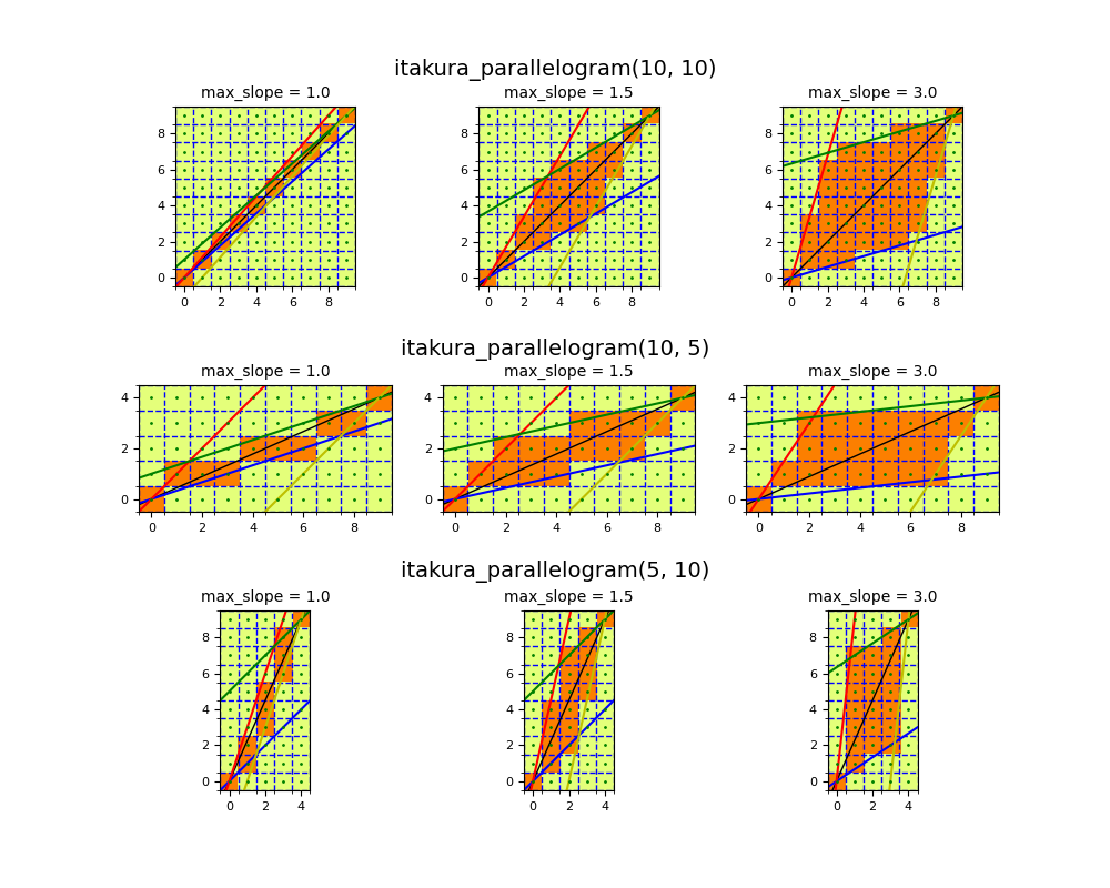
Itakura parallelogram

This example explains how to set the max_slope parameter of the itakura parallelogram when computing the Dynamic Time Warping (DTW) with method == "itakura". The Itakura parallelogram is defined through a max_slope parameter which determines the slope of the steeper side. It is implemented in pyts.metrics.itakura_parallelogram(). The slope of the other side is set to 1 / max_slope. For a feasible region, max_slope must be larger than or equal to 1. This example visualizes the itakura parallelogram with different slopes and temporal dimensions.

# Author: Hicham Janati <hicham.janati@inria.fr>
#         Johann Faouzi <johann.faouzi@gmail.com>
# License: BSD-3-Clause

import numpy as np
import matplotlib.pyplot as plt
from pyts.metrics import itakura_parallelogram
from pyts.metrics.dtw import _get_itakura_slopes

# #####################################################################
# We write a function to visualize the itakura parallelogram for different
# time series lengths.


def plot_itakura(n_timestamps_1, n_timestamps_2, max_slope=1., ax=None):
    """Plot Itakura parallelogram."""
    region = itakura_parallelogram(n_timestamps_1, n_timestamps_2, max_slope)
    max_slope, min_slope = _get_itakura_slopes(
        n_timestamps_1, n_timestamps_2, max_slope)
    mask = np.zeros((n_timestamps_2, n_timestamps_1))
    for i, (j, k) in enumerate(region.T):
        mask[j:k, i] = 1.

    plt.imshow(mask, origin='lower', cmap='Wistia')

    sz = max(n_timestamps_1, n_timestamps_2)
    x = np.arange(-1, sz + 1)

    low_max_line = ((n_timestamps_2 - 1) - max_slope * (n_timestamps_1 - 1)) +\
        max_slope * np.arange(-1, sz + 1)
    up_min_line = ((n_timestamps_2 - 1) - min_slope * (n_timestamps_1 - 1)) +\
        min_slope * np.arange(-1, sz + 1)
    diag = (n_timestamps_2 - 1) / (n_timestamps_1 - 1) * np.arange(-1, sz + 1)
    plt.plot(x, diag, 'black', lw=1)
    plt.plot(x, max_slope * np.arange(-1, sz + 1), 'b', lw=1.5)
    plt.plot(x, min_slope * np.arange(-1, sz + 1), 'r', lw=1.5)
    plt.plot(x, low_max_line, 'g', lw=1.5)
    plt.plot(x, up_min_line, 'y', lw=1.5)

    for i in range(n_timestamps_1):
        for j in range(n_timestamps_2):
            plt.plot(i, j, 'o', color='green', ms=1)

    ax.set_xticks(np.arange(-.5, n_timestamps_1, 1), minor=True)
    ax.set_yticks(np.arange(-.5, n_timestamps_2, 1), minor=True)
    plt.grid(which='minor', color='b', linestyle='--', linewidth=1)
    plt.xticks(np.arange(0, n_timestamps_1, 2))
    plt.yticks(np.arange(0, n_timestamps_2, 2))
    plt.xlim((-0.5, n_timestamps_1 - 0.5))
    plt.ylim((-0.5, n_timestamps_2 - 0.5))


slopes = [1., 1.5, 3.]
rc = {"font.size": 14, "axes.titlesize": 10,
      "xtick.labelsize": 8, "ytick.labelsize": 8}
plt.rcParams.update(rc)


lengths = [(10, 10), (10, 5), (5, 10)]
y_coordinates = [0.915, 0.60, 0.35]

plt.figure(figsize=(10, 8))

for i, ((n1, n2), y) in enumerate(zip(lengths, y_coordinates)):
    for j, slope in enumerate(slopes):
        ax = plt.subplot(3, 3, i * 3 + j + 1)
        plot_itakura(n1, n2, max_slope=slope, ax=ax)
        plt.title('max_slope = {}'.format(slope))
        if j == 1:
            plt.figtext(0.5, y, 'itakura_parallelogram({}, {})'.format(n1, n2),
                        ha='center')
plt.subplots_adjust(hspace=0.4)
plt.show()