pyts.metrics.dtw
-
pyts.metrics.dtw(x=None, y=None, dist='square', method='classic', options=None, precomputed_cost=None, return_cost=False, return_accumulated=False, return_path=False)[source]¶ Dynamic Time Warping (DTW) distance between two samples.
Parameters: - x : array-like, shape = (n_timestamps_1,)
First array. Ignored if
dist == 'precomputed'.- y : array-like, shape = (n_timestamps_2,)
Second array. Ignored if
dist == 'precomputed'.- dist : ‘square’, ‘absolute’, ‘precomputed’ or callable (default = ‘square’)
Distance used. If ‘square’, the squared difference is used. If ‘absolute’, the absolute difference is used. If callable, it must be a function with a numba.njit() decorator that takes as input two numbers (two arguments) and returns a number. If ‘precomputed’,
precomputed_costmust be the cost matrix andmethodmust be ‘classic’, ‘sakoechiba’ or ‘itakura’.- method : str (default = ‘classic’)
Method used. Should be one of
- ‘classic’: (see here)
- ‘sakoechiba’: (see here)
- ‘itakura’: (see here)
- ‘region’: (see here)
- ‘multiscale’: (see here)
- ‘fast’: (see here)
- options : None or dict (default = None)
Dictionary of method options. Here is a quick summary of the available options for each method:
- ‘classic’: None
- ‘sakoechiba’: window_size (int or float)
- ‘itakura’: max_slope (float)
- ‘region’ : region (array-like)
- ‘multiscale’: resolution (int) and radius (int)
- ‘fast’: radius (int)
For more information on these options, see
show_options().- precomputed_cost : array-like, shape = (n_timestamps_1, n_timestamps_2) (default = None)
Precomputed cost matrix between the time series. Ignored if
dist != 'precomputed'.- return_cost : bool (default = False)
If True, the cost matrix is returned.
- return_accumulated : bool (default = False)
If True, the accumulated cost matrix is returned.
- return_path : bool (default = False)
If True, the optimal path is returned.
Returns: - dist : float
The DTW distance between the two arrays.
- cost_mat : ndarray, shape = (n_timestamps_1, n_timestamps_2)
Cost matrix. Only returned if
return_cost=True.- acc_cost_mat : ndarray, shape = (n_timestamps_1, n_timestamps_2)
Accumulated cost matrix. Only returned if
return_accumulated=True.- path : ndarray, shape = (2, path_length)
The optimal path along the cost matrix. The first row consists of the indices of the optimal path for x while the second row consists of the indices of the optimal path for y. Only returned if
return_path=True.
Notes
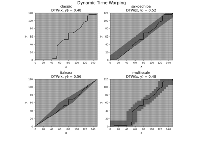
This section describes the available versions of Dynamic Time Warping (DTW) that can be selected by the method parameter.
Unconstrained path
Method ‘classic’ computes the original DTW score between two time series with no constraint region: each cell is a valid cell to find the optimal path minimizing the total cost.
Global constraint region
Using no constraint region allows for very large distortion between both time series, which may be ill-suited for some cases. One possible solution to this issue is to use a global constraint region for the optimal path. A cell can be part of the optimal path if and only if this cell is in the constraint region. Another advantage of using a global constraint region is to decrease the computational complexity to find the optimal path.
Method ‘sakoechiba’ uses a band as the constraint region, allowing for a maximum fixed time shift at every time point.
Method ‘itakura’ uses a parallelogram as the constraint region, allowing for time shifts of varying length: small time shifts at the beginning and at the end of the time series, larger time shifts in the middle.
Adaptative constraint region
One drawback of global constraint regions is that they do not depend on the time series and might be ill-suited for some time series. Adaptative constraint regions are regions that are specific to the two provided time series. However, their computational complexities are larger that the ones of global regions.
Method ‘multiscale’ downsamples both time series by a given factor, computes the optimal path with no constraint region for the downsampled time series, and projects the optimal path on the original scale to define the constraint region.
Method ‘fast’ can be seen as a recursive version of ‘multiscale’: the time series are downsampled so that the new time series are very small, the optimal path for these time series is computed and is projected at the scale that is two times larger. This process is repeated until the original scale of the time series is reached.
References
[1] H. Sakoe and S. Chiba, “Dynamic programming algorithm optimization for spoken word recognition”. IEEE Transactions on Acoustics, Speech, and Signal Processing, 26(1), 43-49 (1978). [2] F. Itakura, “Minimum prediction residual principle applied to speech recognition”. IEEE Transactions on Acoustics, Speech, and Signal Processing, 23(1), 67–72 (1975). [3] M. Müller, H. Mattes and F. Kurth, “An efficient multiscale approach to audio synchronization”. International Conference on Music Information Retrieval, 6(1), 192-197 (2006). [4] S. Salvador ans P. Chan, “FastDTW: Toward Accurate Dynamic Time Warping in Linear Time and Space”. KDD Workshop on Mining Temporal and Sequential Data, 70–80 (2004). Examples
>>> from pyts.metrics import dtw
>>> x = [0, 1, 1]
>>> y = [2, 0, 1]
>>> dtw(x, y, method='sakoechiba', options={'window_size': 0.5})
2.0