10. Multivariate time series

Most of the literature for time series classification is focused on univariate time series. Nonetheless, several algorithms for multivariate time series classification have been published. We also provide simple utilities to extend algorithms for univariate time series to multivariate time series. They can be found in the pyts.multivariate module.

10.1. Classification

MultivariateClassifier extends any classifier for univariate time series to multivariate time series using majority voting: a classifier is fitted for each feature of the multivariate time series, then a majority vote is performed at prediction time.

>>> from pyts.classification import BOSSVS
>>> from pyts.datasets import load_basic_motions
>>> from pyts.multivariate.classification import MultivariateClassifier
>>> X_train, X_test, y_train, y_test = load_basic_motions(return_X_y=True)
>>> clf = MultivariateClassifier(BOSSVS())
>>> clf.fit(X_train, y_train)
MultivariateClassifier(...)
>>> clf.score(X_test, y_test)
1.0

10.2. Transformation

MultivariateTransformer extends any transformer for univariate time series to multivariate time series: a transformer is fitted for each feature of the multivariate time series, then the transformation for each feature is performed. The flatten parameter controls the shape of the output. If each transformation has the same shape, flatten=False does not flatten the output, while flatten=True flattens the output. If some transformations do not have the same shapes, the output is always flattened.

>>> from pyts.datasets import load_basic_motions
>>> from pyts.multivariate.transformation import MultivariateTransformer
>>> from pyts.image import GramianAngularField
>>> X, _, _, _ = load_basic_motions(return_X_y=True)
>>> transformer = MultivariateTransformer(GramianAngularField(),
...                                       flatten=False)
>>> X_new = transformer.fit_transform(X)
>>> X_new.shape
(40, 6, 100, 100)
>>> transformer.set_params(flatten=True)
>>> X_new = transformer.fit_transform(X)
>>> X_new.shape
(40, 60000)

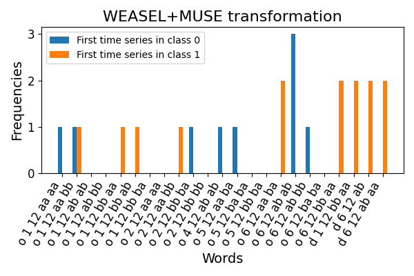
WEASELMUSE is an extension of WEASEL to multivariate time series. It stands for WEASEL plus Multivariate Unsupervised Symbols and dErivatives. It performs an extraction of words for each feature on the original time series and their derivatives and derives their frequencies.

>>> from pyts.datasets import load_basic_motions
>>> from pyts.multivariate.transformation import WEASELMUSE
>>> X_train, X_test, y_train, y_test = load_basic_motions(return_X_y=True)
>>> transformer = WEASELMUSE()
>>> X_new = transformer.fit_transform(X_train, y_train)
>>> X_new.shape
(40, 9086)

Classification can be performed with any standard classifier. In the example below, we use a logistic regression:

>>> from pyts.datasets import load_basic_motions
>>> from pyts.multivariate.transformation import WEASELMUSE
>>> from sklearn.pipeline import make_pipeline
>>> from sklearn.linear_model import LogisticRegression
>>> X_train, X_test, y_train, y_test = load_basic_motions(return_X_y=True)
>>> transformer = WEASELMUSE()
>>> logistic = LogisticRegression(solver='liblinear', multi_class='ovr')
>>> clf = make_pipeline(transformer, logistic)
>>> clf.fit(X_train, y_train)
Pipeline(...)
>>> clf.score(X_test, y_test)
0.975

References

• P. Schäfer, and U. Leser, “Multivariate Time Series Classification with WEASEL+MUSE”. Proceedings of ACM Conference, (2017).

10.3. Image

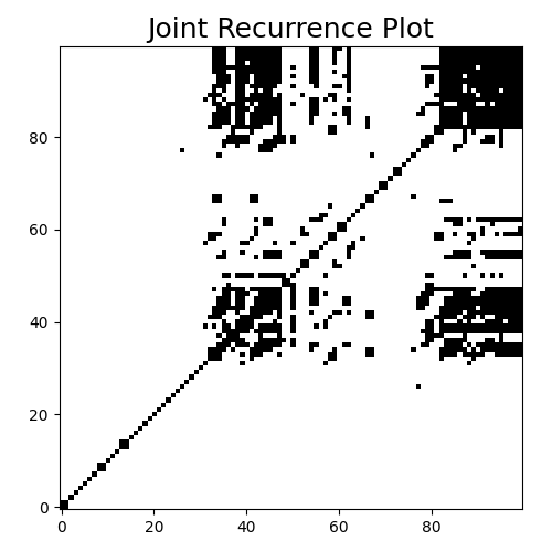
JointRecurrencePlot is an extension of a Recurrence Plot for multivariate time series. For each feature of a multivariate time series, a recurrence plot is constructed. The set of recurrence plots is merged into a single joint recurrence plot using the Hadamard product between all the matrices.

>>> from pyts.datasets import load_basic_motions
>>> from pyts.multivariate.image import JointRecurrencePlot
>>> X, _, _, _ = load_basic_motions(return_X_y=True)
>>> transformer = JointRecurrencePlot()
>>> X_new = transformer.transform(X)
>>> X_new.shape
(40, 100, 100)

References

• M. Romano, M. Thiel, J. Kurths and W. con Bloh, “Multivariate Recurrence Plots”. Physics Letters A (2004)