JointRecurrencePlot

class pyts.multivariate.image.JointRecurrencePlot(dimension: int | float = 1, time_delay: int | float = 1, threshold: float | str | ArrayLike | None = None, percentage: int | float | ArrayLike = 10)

Joint Recurrence Plot.

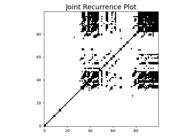
A recurrence plot is an image representing the distances between trajectories extracted from the original time series.

A joint recurrence plot is an extension of recurrence plots for multivariate time series: it is the Hadamard of the recurrence plots obtained for each feature of the multivariate time series.

Parameters:

dimensionint or float (default = 1)

Dimension of the trajectory. If float, it represents a percentage of the size of each time series and must be between 0 and 1.

time_delayint or float (default = 1)

Time gap between two back-to-back points of the trajectory. If float, it represents a percentage of the size of each time series and must be between 0 and 1.

thresholdfloat, ‘point’, ‘distance’ or None or list thereof (default = None)

Threshold for the minimum distance. If None, the recurrence plots are not binarized. If threshold='point', the threshold is computed such as percentage percents of the points are smaller than the threshold. If threshold='distance', the threshold is computed as the percentage of the maximum distance.

percentageint, float or list thereof (default = 10)

Percentage of black points if threshold='point' or percentage of maximum distance for threshold if threshold='distance'. Ignored if threshold is a float or None. Note that the percentage is calculated for each recurrence plot independently, which implies that there will probably be less than percentage percents of black points in the joint recurrence plot.

References

[1]

M. Romano, M. Thiel, J. Kurths and W. con Bloh, “Multivariate Recurrence Plots”. Physics Letters A (2004)

Examples

>>> from pyts.datasets import load_basic_motions
>>> from pyts.multivariate.image import JointRecurrencePlot
>>> X, _, _, _ = load_basic_motions(return_X_y=True)
>>> transformer = JointRecurrencePlot()
>>> X_new = transformer.transform(X)
>>> X_new.shape
(40, 100, 100)

Methods

__init__([dimension, time_delay, threshold, ...])
fit([X, y])	Pass.
fit_transform(X[, y])	Fit to data, then transform it.
get_metadata_routing()	Get metadata routing of this object.
get_params([deep])	Get parameters for this estimator.
set_params(**params)	Set the parameters of this estimator.
transform(X)	Transform each time series into a joint recurrence plot.

__init__(dimension: int | float = 1, time_delay: int | float = 1, threshold: float | str | ArrayLike | None = None, percentage: int | float | ArrayLike = 10) → None

fit(X: ArrayLike | None = None, y: ArrayLike | None = None) → Self

Pass.

Parameters:

X

Ignored

y

Ignored

Returns:

selfobject

transform(X: ArrayLike) → NDArray[float64]

Transform each time series into a joint recurrence plot.

Parameters:

Xarray-like, shape = (n_samples, n_features, n_timestamps)

Multivariate time series.

Returns:

X_newarray, shape = (n_samples, image_size, image_size)

Joint Recurrence plots. image_size is the number of trajectories and is equal to n_timestamps - (dimension - 1) * time_delay.

Examples using pyts.multivariate.image.JointRecurrencePlot

Joint Recurrence Plot

Joint Recurrence Plot