4. Imaging time series
Imaging time series, that is transforming time series into images, is another
popular transformation. One important upside of this transformation is retrieving
information for any pair of time points  given a time series
 .
Deep neural networks, especially convolutional neural networks, have been
used to classify these imaged time series. While pyts does not provide
deep neural networks, it provides algorithms to transform time series into
images in the
.
Deep neural networks, especially convolutional neural networks, have been
used to classify these imaged time series. While pyts does not provide
deep neural networks, it provides algorithms to transform time series into
images in the pyts.image module.
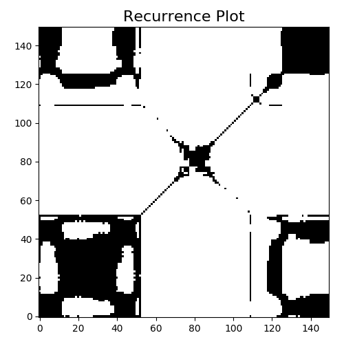
4.1. Recurrence Plot
RecurrencePlot extracts trajectories from time series and computes the
pairwise distances between these trajectories. The trajectories are defined
as:

where  is the
 dimension of the trajectories and  is the
 time_delay. The recurrence plot, denoted  , is the
binarized pairwise distance matrix between the trajectories:
, is the
binarized pairwise distance matrix between the trajectories:

where  is the Heaviside function and
  is the
 threshold. Different strategies can be used to choose the threshold,
such as a given float or a quantile of the distances.
>>> from pyts.datasets import load_gunpoint
>>> from pyts.image import RecurrencePlot
>>> X, _, _, _ = load_gunpoint(return_X_y=True)
>>> transformer = RecurrencePlot()
>>> X_new = transformer.transform(X)
>>> X_new.shape
(50, 150, 150)
Images can be flattened by setting the flatten parameter to True,
so that classification can be directly performed:
>>> from pyts.image import RecurrencePlot
>>> from pyts.datasets import load_gunpoint
>>> from sklearn.pipeline import make_pipeline
>>> from sklearn.linear_model import LogisticRegression
>>> X_train, X_test, y_train, y_test = load_gunpoint(return_X_y=True)
>>> recurrence = RecurrencePlot(dimension=15, time_delay=3, flatten=True)
>>> logistic = LogisticRegression(solver='liblinear')
>>> clf = make_pipeline(recurrence, logistic)
>>> clf.fit(X_train, y_train)
Pipeline(...)
>>> clf.score(X_test, y_test)
0.933...
References
- J.-P Eckmann, S. Oliffson Kamphorst and D Ruelle, “Recurrence Plots of Dynamical Systems”. Europhysics Letters (1987).
- N. Hatami, Y. Gavet and J. Debayle, “Classification of Time-Series Images Using Deep Convolutional Neural Networks”. https://arxiv.org/abs/1710.00886
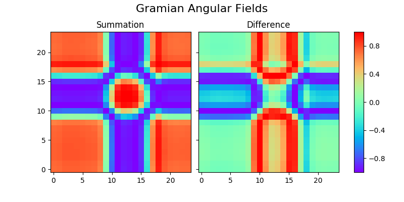
4.2. Gramian Angular Field
GramianAngularField creates a matrix of temporal correlations for each
. First it rescales the time series in a range ![[a, b]](../_images/math/81020ad941964580fece7ab05b36d0c51847489d.svg) where
where  . Then it computes the polar coordinates of
the scaled time series by taking the
. Then it computes the polar coordinates of
the scaled time series by taking the  . Finally it computes the
cosine of the sum of the angles for the Gramian Angular Summation Field
(GASF) or the sine of the difference of the angles for the Gramian Angular
Difference Field (GADF).
. Finally it computes the
cosine of the sum of the angles for the Gramian Angular Summation Field
(GASF) or the sine of the difference of the angles for the Gramian Angular
Difference Field (GADF).

The method parameter controls which type of Gramian angular fields are
computed.
>>> from pyts.datasets import load_gunpoint
>>> from pyts.image import GramianAngularField
>>> X, _, _, _ = load_gunpoint(return_X_y=True)
>>> transformer = GramianAngularField()
>>> X_new = transformer.transform(X)
>>> X_new.shape
(50, 150, 150)
Images can be flattened by setting the flatten parameter to True,
so that classification can be directly performed:
>>> from pyts.image import GramianAngularField
>>> from pyts.datasets import load_gunpoint
>>> from sklearn.pipeline import make_pipeline
>>> from sklearn.linear_model import LogisticRegression
>>> X_train, X_test, y_train, y_test = load_gunpoint(return_X_y=True)
>>> gaf = GramianAngularField(flatten=True)
>>> logistic = LogisticRegression(solver='liblinear')
>>> clf = make_pipeline(gaf, logistic)
>>> clf.fit(X_train, y_train)
Pipeline(...)
>>> clf.score(X_test, y_test)
0.973...
References
- Z. Wang and T. Oates, “Encoding Time Series as Images for Visual Inspection and Classification Using Tiled Convolutional Neural Networks.” AAAI Workshop (2015).
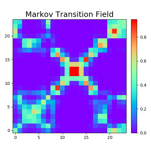
4.3. Markov Transition Field
MarkovTransitionField discretizes a time series into bins.
It then computes the Markov Transition Matrix of the discretized time series.
Finally it spreads out the transition matrix to a field in order to reduce
the loss of temporal information.
>>> from pyts.datasets import load_gunpoint
>>> from pyts.image import MarkovTransitionField
>>> X, _, _, _ = load_gunpoint(return_X_y=True)
>>> transformer = MarkovTransitionField()
>>> X_new = transformer.transform(X)
>>> X_new.shape
(50, 150, 150)
Images can be flattened by setting the flatten parameter to True,
so that classification can be directly performed:
>>> from pyts.image import MarkovTransitionField
>>> from pyts.datasets import load_gunpoint
>>> from sklearn.pipeline import make_pipeline
>>> from sklearn.linear_model import LogisticRegression
>>> X_train, X_test, y_train, y_test = load_gunpoint(return_X_y=True)
>>> mtf = MarkovTransitionField(image_size=0.1, n_bins=3, flatten=True)
>>> logistic = LogisticRegression(solver='liblinear')
>>> clf = make_pipeline(mtf, logistic)
>>> clf.fit(X_train, y_train)
Pipeline(...)
>>> clf.score(X_test, y_test)
0.92
References
- Z. Wang and T. Oates, “Encoding Time Series as Images for Visual Inspection and Classification Using Tiled Convolutional Neural Networks.” AAAI Workshop (2015).
