pyts.image.RecurrencePlot
-
class
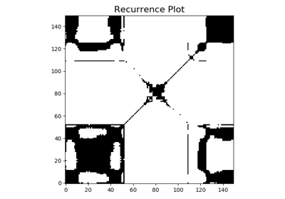
pyts.image.RecurrencePlot(dimension=1, time_delay=1, threshold=None, percentage=10, flatten=False)[source]¶ Recurrence Plot.
A recurrence plot is an image representing the distances between trajectories extracted from the original time series.
Parameters: - dimension : int or float (default = 1)
Dimension of the trajectory. If float, If float, it represents a percentage of the size of each time series and must be between 0 and 1.
- time_delay : int or float (default = 1)
Time gap between two back-to-back points of the trajectory. If float, If float, it represents a percentage of the size of each time series and must be between 0 and 1.
- threshold : float, ‘point’, ‘distance’ or None (default = None)
Threshold for the minimum distance. If None, the recurrence plots are not binarized. If ‘point’, the threshold is computed such as percentage percents of the points are smaller than the threshold. If ‘distance’, the threshold is computed as the percentage of the maximum distance.
- percentage : int or float (default = 10)
Percentage of black points if
threshold='point'or percentage of maximum distance for threshold ifthreshold='distance'. Ignored ifthresholdis a float or None.- flatten : bool (default = False)
If True, images are flattened to be one-dimensional.
Notes
Given a time series
 , the extracted
trajectories are
, the extracted
trajectories are
where
 is the
 dimensionof the trajectories and is the
 time_delay. The recurrence plot, denoted , is the
pairwise distance between the trajectories
, is the
pairwise distance between the trajectories
where
 is the Heaviside function and
  is the
 threshold.References
[Rc0c3bc29e8b8-1] J.-P Eckmann, S. Oliffson Kamphorst and D Ruelle, “Recurrence Plots of Dynamical Systems”. Europhysics Letters (1987). Examples
>>> from pyts.datasets import load_gunpoint
>>> from pyts.image import RecurrencePlot
>>> X, _, _, _ = load_gunpoint(return_X_y=True)
>>> transformer = RecurrencePlot()
>>> X_new = transformer.transform(X)
>>> X_new.shape
(50, 150, 150)
Methods
__init__(self[, dimension, time_delay, …])Initialize self. fit(self[, X, y])Pass. fit_transform(self, X[, y])Fit to data, then transform it. get_params(self[, deep])Get parameters for this estimator. set_params(self, \*\*params)Set the parameters of this estimator. transform(self, X)Transform each time series into a recurrence plot. -
__init__(self, dimension=1, time_delay=1, threshold=None, percentage=10, flatten=False)[source]¶ Initialize self. See help(type(self)) for accurate signature.
-
fit_transform(self, X, y=None, **fit_params)¶ Fit to data, then transform it.
Fits transformer to X and y with optional parameters fit_params and returns a transformed version of X.
Parameters: - X : numpy array of shape [n_samples, n_features]
Training set.
- y : numpy array of shape [n_samples]
Target values.
- **fit_params : dict
Additional fit parameters.
Returns: - X_new : numpy array of shape [n_samples, n_features_new]
Transformed array.
-
get_params(self, deep=True)¶ Get parameters for this estimator.
Parameters: - deep : bool, default=True
If True, will return the parameters for this estimator and contained subobjects that are estimators.
Returns: - params : mapping of string to any
Parameter names mapped to their values.
-
set_params(self, **params)¶ Set the parameters of this estimator.
The method works on simple estimators as well as on nested objects (such as pipelines). The latter have parameters of the form
<component>__<parameter>so that it’s possible to update each component of a nested object.Parameters: - **params : dict
Estimator parameters.
Returns: - self : object
Estimator instance.
-
transform(self, X)[source]¶ Transform each time series into a recurrence plot.
Parameters: - X : array-like, shape = (n_samples, n_timestamps)
Returns: - X_new : array, shape = (n_samples, image_size, image_size)
Recurrence plots.
image_sizeis the number of trajectories and is equal ton_timestamps - (dimension - 1) * time_delay. Ifflatten=True, the shape is (n_samples, image_size * image_size).