3. Extracting features from time series

Standard machine learning algorithms are not always well suited for raw time series because they cannot capture the high correlation between consecutive time points: treating time points as features may not be optimal. Therefore, algorithms that extract features from time series have been developed. These algorithms transforms a dataset of time series with shape (n_samples, n_timestamps) into a dataset of features with shape (n_samples, n_extracted_features) that can be used to fit a standard classifier. They can be found in the pyts.transformation module. The following sections describe the algorithms made available.

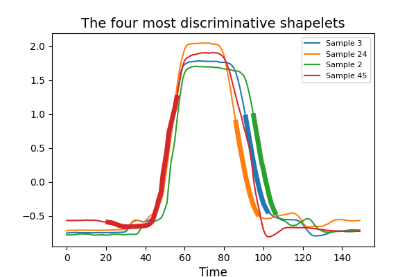
3.1. ShapeletTransform

ShapeletTransform is a shapelet-based approach to extract features. A shapelet is defined as a contiguous subsequence of a time series. The distance between a shapelet and a time series is defined as the minimum of the distances between this shapelet and all the shapelets of identical length extracted from this time series. ShapeletTransform extracts the n_shapelets most discriminative shapelets given a criterion (mutual information or F-scores) from a dataset of time series when fit is called. The indices of the selected shapelets are made available via the indices_ attribute.

ShapeletTransform derives the distances between the selected shapelets and a dataset of time series when transform is called. fit_transform is an optimized version of fit followed by transform since the distances between the shapelets and the time series must be computed when fit is called:

>>> from pyts.transformation import ShapeletTransform
>>> X = [[0, 2, 3, 4, 3, 2, 1],
...      [0, 1, 3, 4, 3, 4, 5],
...      [2, 1, 0, 2, 1, 5, 4],
...      [1, 2, 2, 1, 0, 3, 5]]
>>> y = [0, 0, 1, 1]
>>> st = ShapeletTransform(n_shapelets=2, window_sizes=[3])
>>> X_new = st.fit_transform(X, y)
>>> X_new.shape()
(4, 2)

Classification can be performed with any standard classifier. In the example below, we use a Support Vector Machine with a linear kernel:

>>> import numpy as np
>>> from pyts.transformation import ShapeletTransform
>>> from pyts.datasets import load_gunpoint
>>> from sklearn.pipeline import make_pipeline
>>> from sklearn.svm import LinearSVC
>>> X_train, X_test, y_train, y_test = load_gunpoint(return_X_y=True)
>>> shapelet = ShapeletTransform(window_sizes=np.arange(10, 130, 3), random_state=42)
>>> svc = LinearSVC()
>>> clf = make_pipeline(shapelet, svc)
>>> clf.fit(X_train, y_train)
Pipeline(...)
>>> clf.score(X_test, y_test)
0.966...

References

• J. Lines, L. M. Davis, J. Hills and A. Bagnall, “A Shapelet Transform for Time Series Classification”. Data Mining and Knowledge Discovery, 289-297 (2012).

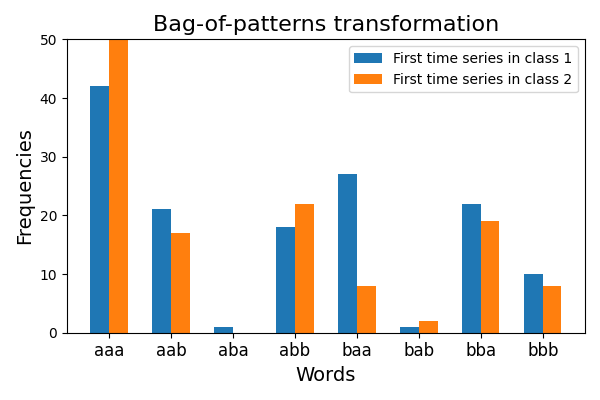
3.2. BagOfPatterns

BagOfPatterns is built on top of the Bag of words. transformation. First it transforms each time series into a bag of words, then the frequency of each word for each time series is computed. Therefore, it transforms each time series into a histogram. The vocabulary_ attribute is a mapping from the feature indices to the corresponding words.

Classification can be performed with any standard classifier. In the example below, we use a k-nearest neighbors classifier with the Euclidean distance:

>>> from pyts.transformation import BagOfPatterns
>>> from pyts.datasets import load_gunpoint
>>> from sklearn.neighbors import KNeighborsClassifier
>>> from sklearn.pipeline import make_pipeline
>>> X_train, X_test, y_train, y_test = load_gunpoint(return_X_y=True)
>>> clf = make_pipeline(
...    BagOfPatterns(window_size=32, word_size=4, n_bins=4,
                     strategy='normal', numerosity_reduction=False),
...    KNeighborsClassifier(n_neighbors=1)
... )
>>> clf.fit(X_train, y_train)
>>> clf.score(X_test, y_test)
0.98

References

• J. Lin, R. Khade and Y. Li, “Rotation-invariant similarity in time series using bag-of-patterns representation”. Journal of Intelligent Information Systems, 39 (2), 287-315 (2012).

3.3. BOSS

BOSS stands for Bag Of Symbolic-Fourier-Approximation Symbols. BOSS extracts words from time series using the Symbolic Fourier Approximation algorithm and derives their frequencies for each time series.

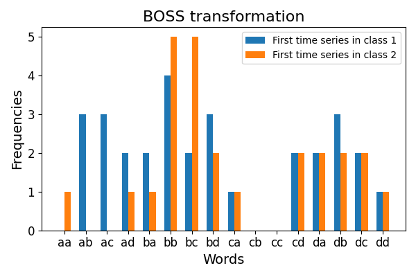
The vocabulary_ attribute is a mapping from the feature indices to the corresponding words:

>>> from pyts.datasets import load_gunpoint
>>> from pyts.transformation import BOSS
>>> X_train, X_test, _, _ = load_gunpoint(return_X_y=True)
>>> boss = BOSS(word_size=2, n_bins=2, sparse=False)
>>> boss.fit(X_train)
BOSS(...)
>>> sorted(boss.vocabulary_.values())
['aa', 'ab', 'ba', 'bb']
>>> boss.transform(X_test)
array(...)

Classification can be performed with any standard classifier. In the example below, we use a k-nearest neighbors classifier with the pyts.metrics.boss() metric:

>>> from pyts.datasets import load_gunpoint
>>> from pyts.transformation import BOSS
>>> from pyts.classification import KNeighborsClassifier
>>> from sklearn.pipeline import make_pipeline
>>> X_train, X_test, y_train, y_test = load_gunpoint(return_X_y=True)
>>> boss = BOSS(word_size=8, window_size=40, norm_mean=True, drop_sum=True, sparse=False)
>>> knn = KNeighborsClassifier(metric='boss')
>>> clf = make_pipeline(boss, knn)
>>> clf.fit(X_train, y_train)
Pipeline(...)
>>> clf.score(X_test, y_test)
1.0

References

• P. Schäfer, “The BOSS is concerned with time series classification in the presence of noise”. Data Mining and Knowledge Discovery, 29(6), 1505-1530 (2015).

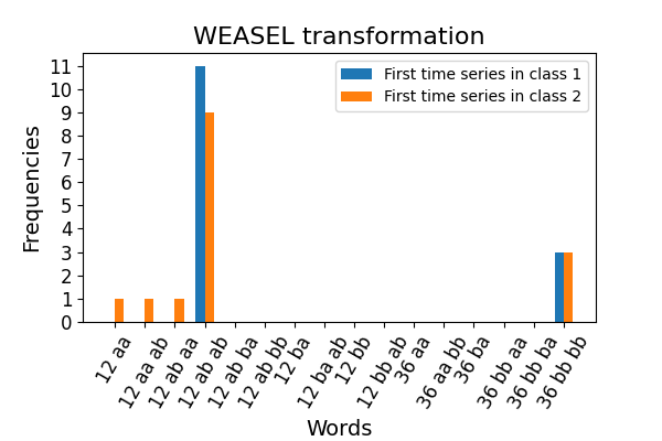
3.4. WEASEL

WEASEL stands for Word ExtrAction for time SEries cLassification. While BOSS extracts words with a single sliding window, WEASEL extracts words with several sliding windows of different sizes, and selects the most discriminative words according to the chi-squared test. The vocabulary_ attribute is a mapping from the feature indices to the corresponding words.

For new input data, the frequencies of each selected word are derived:

>>> from pyts.datasets import load_gunpoint
>>> from pyts.transformation import WEASEL
>>> X_train, X_test, y_train, _ = load_gunpoint(return_X_y=True)
>>> weasel = WEASEL(sparse=False)
>>> weasel.fit(X_train, y_train)
WEASEL(...)
>>>len(weasel.vocabulary_)
73
>>> weasel.transform(X_test).shape
(150, 73)

Classification can be performed with any standard classifier. In the example below, we use a logistic regression:

>>> import numpy as np
>>> from pyts.transformation import WEASEL
>>> from pyts.datasets import load_gunpoint
>>> from sklearn.pipeline import make_pipeline
>>> from sklearn.linear_model import LogisticRegression
>>> X_train, X_test, y_train, y_test = load_gunpoint(return_X_y=True)
>>> weasel = WEASEL(word_size=4, window_sizes=np.arange(5, 149))
>>> logistic = LogisticRegression(solver='liblinear')
>>> clf = make_pipeline(weasel, logistic)
>>> clf.fit(X_train, y_train)
Pipeline(...)
>>> clf.score(X_test, y_test)
0.96

References

• P. Schäfer, and U. Leser, “Fast and Accurate Time Series Classification with WEASEL”. Conference on Information and Knowledge Management, 637-646 (2017).

3.5. ROCKET

ROCKET stands for RandOm Convolutional KErnel Transform. ROCKET generates a great variety of random convolutional kernels and extracts two features from the convolutions: the maximum and the proportion of positive values. The kernels are generated randomly and are not learned, which greatly speeds up the computation of this transformation.

>>> from pyts.datasets import load_gunpoint
>>> from pyts.transformation import ROCKET
>>> X_train, X_test, _, _ = load_gunpoint(return_X_y=True)
>>> rocket = ROCKET()
>>> rocket.fit(X_train)
ROCKET(...)
>>> rocket.transform(X_train).shape
(50, 20000)
>>> rocket.transform(X_test).shape
(150, 20000)

References

• A. Dempster, F. Petitjean and G. I. Webb, “ROCKET: Exceptionally fast and accurate time series classification using random convolutional kernels”. Data Mining and Knowledge Discovery, 34(5), 1454-1495 (2020).