2. Classification of raw time series
Algorithms that can directly classify time series have been developed.
The following sections will describe the ones that are available in pyts.
They can be found in the pyts.classification module.
2.1. KNeighborsClassifier
The k-nearest neighbors algorithm is a relatively simple algorithm.
KNeighborsClassifier finds the k nearest neighbors of a time series
and the predicted class is determined with majority voting. A key parameter
of this algorithm is the metric used to find the nearest neighbors.
A popular metric for time series is the Dynamic Time Warping metric
(see Metrics for time series).
The one-nearest-neighbor algorithm with this metric can be considered as
a good baseline for time series classification:
>>> from pyts.classification import KNeighborsClassifier
>>> from pyts.datasets import load_gunpoint
>>> X_train, X_test, y_train, y_test = load_gunpoint(return_X_y=True)
>>> clf = KNeighborsClassifier(metric='dtw')
>>> clf.fit(X_train, y_train)
KNeighborsClassifier(...)
>>> clf.score(X_test, y_test)
0.91...
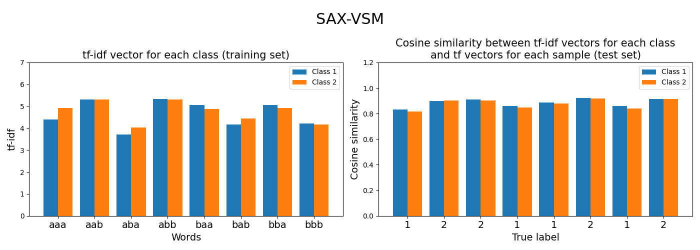
2.2. SAXVSM
SAX-VSM stands for Symbolic Aggregate approXimation in
Vector Space Model.
SAXVSM is an algorithm based on the SAX representation of time
series in a vector space model. Subsequences are extracted using a sliding
window and each subsequence of real numbers is transformed into a word
(i.e., a sequence of symbols) using the Symbolic Aggregate approXimation algorithm.
Each time series is thus transformed into a bag of words (the order of the
words is not taken into account). For each class, all the bags of words from
all the time series belonging to this class are combined into a single bag of
words, leading to a bag of words for each class.
Finally, a term-frequency inverse-term-frequency (tf-idf) vector is computed
for each class. Predictions are made using the cosine similarity between
the time series and the tf-idf vectors for each class. The predicted class
is the class yielding the highest cosine similarity.
>>> from pyts.classification import SAXVSM
>>> from pyts.datasets import load_gunpoint
>>> X_train, X_test, y_train, y_test = load_gunpoint(return_X_y=True)
>>> clf = SAXVSM(window_size=34, sublinear_tf=False, use_idf=False)
>>> clf.fit(X_train, y_train)
SAXVSM(...)
>>> clf.score(X_test, y_test)
0.76
References
- P. Senin, and S. Malinchik, “SAX-VSM: Interpretable Time Series Classification Using SAX and Vector Space Model”. International Conference on Data Mining, 13, 1175-1180 (2013).
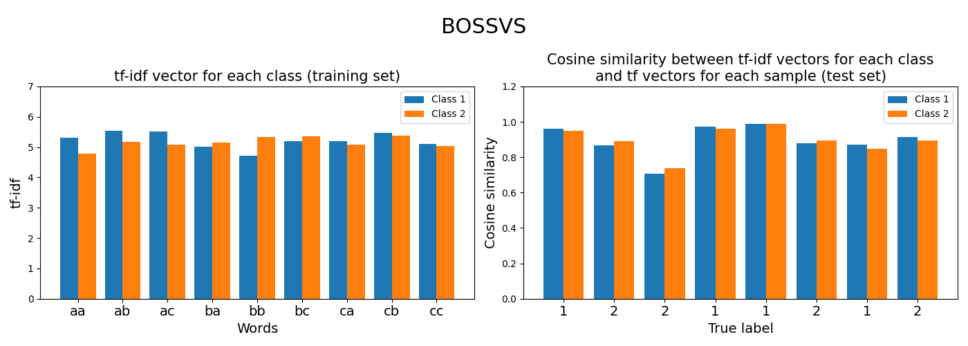
2.3. BOSSVS
BOSSVS stands for Bag of Symbolic Fourier Symbols in
Vector Space.
BOSSVS is another bag-of-words approach for time series classification.
BOSSVS is relatively similar to SAX-VSM: it builds a term-frequency
inverse-term-frequency vector for each class, but the symbols used to create
the words are generated with the Symbolic Fourier Approximation algorithm.
>>> from pyts.classification import BOSSVS
>>> from pyts.datasets import load_gunpoint
>>> X_train, X_test, y_train, y_test = load_gunpoint(return_X_y=True)
>>> clf = BOSSVS(window_size=28)
>>> clf.fit(X_train, y_train)
BOSSVS(...)
>>> clf.score(X_test, y_test)
0.98
References
- P. Schäfer, “Scalable Time Series Classification”. Data Mining and Knowledge Discovery, 30(5), 1273-1298 (2016).
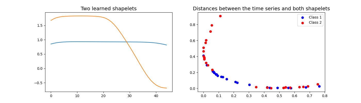
2.4. LearningShapelets
LearningShapelets is a shapelet-based classifier.
A shapelet is defined as a contiguous subsequence of a time series.
The distance between a shapelet and a time series is defined as the minimum
of the distances between this shapelet and all the shapelets of identical
length extracted from this time series.
This estimator consists of two steps: computing the distances between the
shapelets and the time series, then computing a logistic regression using
these distances as features. This algorithm learns the shapelets as well as
the coefficients of the logistic regression.
>>> from pyts.classification import LearningShapelets
>>> from pyts.datasets import load_gunpoint
>>> X_train, X_test, y_train, y_test = load_gunpoint(return_X_y=True)
>>> clf = LearningShapelets(random_state=42, tol=0.01)
>>> clf.fit(X_train, y_train)
LearningShapelets(...)
>>> clf.score(X_test, y_test)
0.766...
References
- J. Grabocka, N. Schilling, M. Wistuba and L. Schmidt-Thieme, “Learning Time-Series Shapelets”. International Conference on Data Mining, 14, 392-401 (2014).
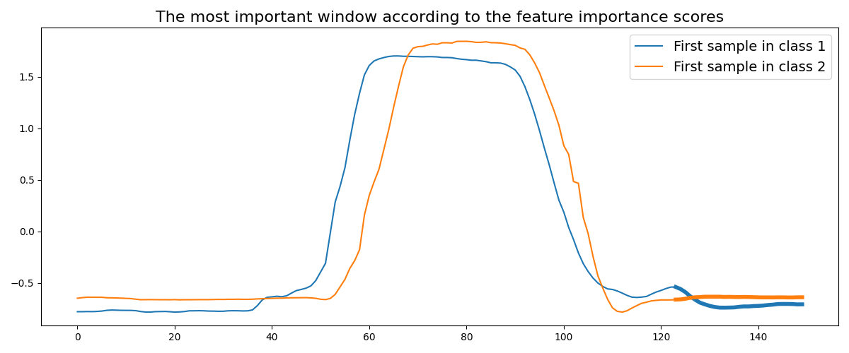
2.5. TimeSeriesForest
TimeSeriesForest is a two-stage algorithm. First it extracts three
features from a given number of windows: the mean, the standard deviation and
the slope of the simple linear regression. Then a random forest is fitted using
the extracted features as input data. These three statistics are fast to
compute and give a lot of information about the window. The windows are
generated randomly and the number of windows is controlled with the
n_windows parameter. Using the feature importance scores of the random
forest, one can easily find the most important windows to classify time series.
>>> from pyts.datasets import load_gunpoint
>>> from pyts.classification import TimeSeriesForest
>>> X_train, X_test, y_train, y_test = load_gunpoint(return_X_y=True)
>>> clf = TimeSeriesForest(random_state=43)
>>> clf.fit(X_train, y_train)
TimeSeriesForest(...)
>>> clf.score(X_test, y_test)
0.973333...
References
- H. Deng, G. Runger, E. Tuv and M. Vladimir, “A Time Series Forest for Classification and Feature Extraction”. Information Sciences, 239, 142-153 (2013).
2.6. Time Series Bag-of-Features
TSBF (acronym for Time Series Bag-of-Features) is a complex algorithm
whose fitting procedure consists of the following steps:
- Random intervals are generated.
- Each interval is split into several subintervals.
- Three features are extracted from each subinterval: the mean, the standard deviation and the slope.
- Four features are also extracted from the whole interval: the mean, the standard deviation and the start and end indices.
- A first random forest classifier is fitted on this dataset of subsequences, and the label of a subsequence is given by the label of the time series from which this subsequence has been extracted.
- Out-of-bag probabilities for each class are binned across all the subsequences extracted from a given time series; the mean probability for each class is also computed. They are the features extracted from the original data set.
- A second random forest classifier is finally fitted using these extracted features.
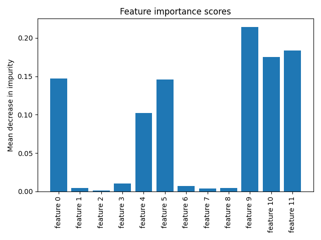
Since the final estimator is a random forest classifier, one can extract the feature importance scores:
>>> from pyts.datasets import load_gunpoint
>>> from pyts.classification import TimeSeriesForest
>>> X_train, X_test, y_train, y_test = load_gunpoint(return_X_y=True)
>>> clf = TimeSeriesForest(random_state=43)
>>> clf.fit(X_train, y_train)
TimeSeriesForest(...)
>>> clf.score(X_test, y_test)
0.973333...
References
- M.G. Baydogan, G. Runger and E. Tuv, “A Bag-of-Features Framework to Classify Time Series”. IEEE Transactions on Pattern Analysis and Machine Intelligence, 35(11), 2796-2802 (2013).
