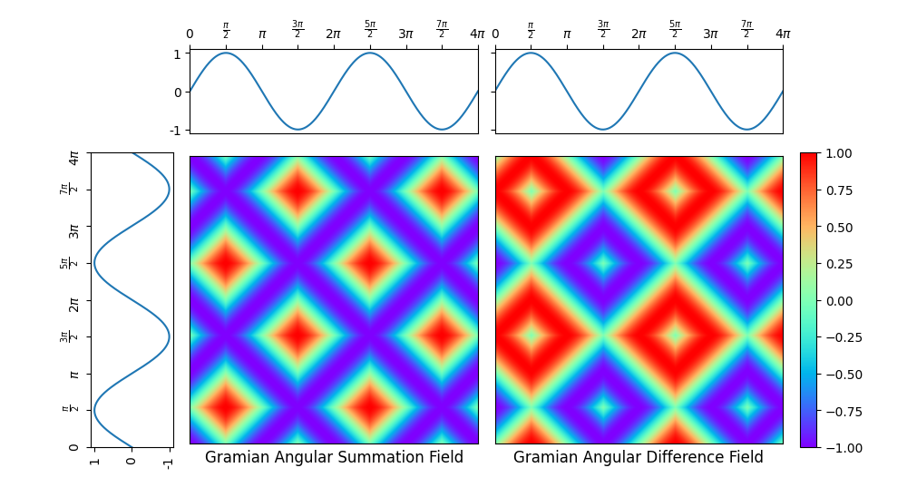
Single Gramian angular field

A Gramian angular field is an image obtained from a time series, representing some kind of temporal correlation between each pair of values from the time series. Two methods are available: Gramian angular summation field and Gramian angular difference field. It is implemented as pyts.image.GramianAngularField.

In this example, the considered time series is the sequence of the sine function values for 1000 equally-spaced points in the interval . Both the corresponding Gramnian angular summation and difference fields are plotted.

Since the API is designed for machine learning, the transform() method of the pyts.image.GramianAngularField class expects a data set of time series as input, so the time series is transformed into a data set with a single time series (X = np.array([x])) and the first element of the data set of Gramian angular fields is retrieved (ax_gasf.imshow(X_gasf[0], ...).

# Author: Johann Faouzi <johann.faouzi@gmail.com>
# License: BSD-3-Clause

import numpy as np
import matplotlib.pyplot as plt
from pyts.image import GramianAngularField


# Create a toy time series using the sine function
time_points = np.linspace(0, 4 * np.pi, 1000)
x = np.sin(time_points)
X = np.array([x])

# Compute Gramian angular fields
gasf = GramianAngularField(method='summation')
X_gasf = gasf.fit_transform(X)

gadf = GramianAngularField(method='difference')
X_gadf = gadf.fit_transform(X)

# Plot the time series and its recurrence plot
width_ratios = (2, 7, 7, 0.4)
height_ratios = (2, 7)
width = 10
height = width * sum(height_ratios) / sum(width_ratios)
fig = plt.figure(figsize=(width, height))
gs = fig.add_gridspec(2, 4,  width_ratios=width_ratios,
                      height_ratios=height_ratios,
                      left=0.1, right=0.9, bottom=0.1, top=0.9,
                      wspace=0.1, hspace=0.1)

# Define the ticks and their labels for both axes
time_ticks = np.linspace(0, 4 * np.pi, 9)
time_ticklabels = [r'$0$', r'$\frac{\pi}{2}$', r'$\pi$',
                   r'$\frac{3\pi}{2}$', r'$2\pi$', r'$\frac{5\pi}{2}$',
                   r'$3\pi$', r'$\frac{7\pi}{2}$', r'$4\pi$']
value_ticks = [-1, 0, 1]
reversed_value_ticks = value_ticks[::-1]

# Plot the time series on the left with inverted axes
ax_left = fig.add_subplot(gs[1, 0])
ax_left.plot(x, time_points)
ax_left.set_xticks(reversed_value_ticks)
ax_left.set_xticklabels(reversed_value_ticks, rotation=90)
ax_left.set_yticks(time_ticks)
ax_left.set_yticklabels(time_ticklabels, rotation=90)
ax_left.set_ylim((0, 4 * np.pi))
ax_left.invert_xaxis()

# Plot the time series on the top
ax_top1 = fig.add_subplot(gs[0, 1])
ax_top2 = fig.add_subplot(gs[0, 2])
for ax in (ax_top1, ax_top2):
    ax.plot(time_points, x)
    ax.set_xticks(time_ticks)
    ax.set_xticklabels(time_ticklabels)
    ax.set_yticks(value_ticks)
    ax.xaxis.tick_top()
    ax.set_xlim((0, 4 * np.pi))
ax_top1.set_yticklabels(value_ticks)
ax_top2.set_yticklabels([])

# Plot the Gramian angular fields on the bottom right
ax_gasf = fig.add_subplot(gs[1, 1])
ax_gasf.imshow(X_gasf[0], cmap='rainbow', origin='lower',
               extent=[0, 4 * np.pi, 0, 4 * np.pi])
ax_gasf.set_xticks([])
ax_gasf.set_yticks([])
ax_gasf.set_title('Gramian Angular Summation Field', y=-0.09)

ax_gadf = fig.add_subplot(gs[1, 2])
im = ax_gadf.imshow(X_gadf[0], cmap='rainbow', origin='lower',
                    extent=[0, 4 * np.pi, 0, 4 * np.pi])
ax_gadf.set_xticks([])
ax_gadf.set_yticks([])
ax_gadf.set_title('Gramian Angular Difference Field', y=-0.09)

# Add colorbar
ax_cbar = fig.add_subplot(gs[1, 3])
fig.colorbar(im, cax=ax_cbar)

plt.show()