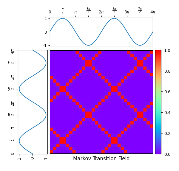
Single Markov transition field

A Markov transition field is an image obtained from a time series, representing a field of transition probabilities for a discretized time series. Different strategies can be used to bin time series. It is implemented as pyts.image.MarkovTransitionField.

In this example, the considered time series is the sequence of the sine function values for 1000 equally-spaced points in the interval . One can see on the Markov transition field that the sine function is periodic with period and smooth (only neighbor bins have a positive transition probability).

Since the API is designed for machine learning, the transform() method of the pyts.image.MarkovTransitionField class expects a data set of time series as input, so the time series is transformed into a data set with a single time series (X = np.array([x])) and the first element of the data set of Gramian angular fields is retrieved (ax_mtf.imshow(X_mtf[0], ...).

# Author: Johann Faouzi <johann.faouzi@gmail.com>
# License: BSD-3-Clause

import numpy as np
import matplotlib.pyplot as plt
from pyts.image import MarkovTransitionField


# Create a toy time series using the sine function
time_points = np.linspace(0, 4 * np.pi, 1000)
x = np.sin(time_points)
X = np.array([x])

# Compute Gramian angular fields
mtf = MarkovTransitionField(n_bins=8)
X_mtf = mtf.fit_transform(X)

# Plot the time series and its Markov transition field
width_ratios = (2, 7, 0.4)
height_ratios = (2, 7)
width = 6
height = width * sum(height_ratios) / sum(width_ratios)
fig = plt.figure(figsize=(width, height))
gs = fig.add_gridspec(2, 3,  width_ratios=width_ratios,
                      height_ratios=height_ratios,
                      left=0.1, right=0.9, bottom=0.1, top=0.9,
                      wspace=0.05, hspace=0.05)

# Define the ticks and their labels for both axes
time_ticks = np.linspace(0, 4 * np.pi, 9)
time_ticklabels = [r'$0$', r'$\frac{\pi}{2}$', r'$\pi$',
                   r'$\frac{3\pi}{2}$', r'$2\pi$', r'$\frac{5\pi}{2}$',
                   r'$3\pi$', r'$\frac{7\pi}{2}$', r'$4\pi$']
value_ticks = [-1, 0, 1]
reversed_value_ticks = value_ticks[::-1]

# Plot the time series on the left with inverted axes
ax_left = fig.add_subplot(gs[1, 0])
ax_left.plot(x, time_points)
ax_left.set_xticks(reversed_value_ticks)
ax_left.set_xticklabels(reversed_value_ticks, rotation=90)
ax_left.set_yticks(time_ticks)
ax_left.set_yticklabels(time_ticklabels, rotation=90)
ax_left.set_ylim((0, 4 * np.pi))
ax_left.invert_xaxis()

# Plot the time series on the top
ax_top = fig.add_subplot(gs[0, 1])
ax_top.plot(time_points, x)
ax_top.set_xticks(time_ticks)
ax_top.set_xticklabels(time_ticklabels)
ax_top.set_yticks(value_ticks)
ax_top.set_yticklabels(value_ticks)
ax_top.xaxis.tick_top()
ax_top.set_xlim((0, 4 * np.pi))
ax_top.set_yticklabels(value_ticks)

# Plot the Gramian angular fields on the bottom right
ax_mtf = fig.add_subplot(gs[1, 1])
im = ax_mtf.imshow(X_mtf[0], cmap='rainbow', origin='lower', vmin=0., vmax=1.,
                   extent=[0, 4 * np.pi, 0, 4 * np.pi])
ax_mtf.set_xticks([])
ax_mtf.set_yticks([])
ax_mtf.set_title('Markov Transition Field', y=-0.09)

# Add colorbar
ax_cbar = fig.add_subplot(gs[1, 2])
fig.colorbar(im, cax=ax_cbar)

plt.show()