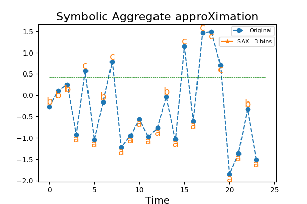
Symbolic Aggregate approXimation

Binning continuous data into intervals can be seen as an approximation that reduces noise and captures the trend of a time series. The Symbolic Aggregate approXimation (SAX) algorithm bins continuous time series into intervals, transforming independently each time series (a sequence of floats) into a sequence of symbols, usually letters. This example illustrates the transformation. It is implemented as pyts.approximation.SymbolicAggregateApproximation.

# Author: Johann Faouzi <johann.faouzi@gmail.com>
# License: BSD-3-Clause

import numpy as np
import matplotlib.lines as mlines
import matplotlib.pyplot as plt
from scipy.stats import norm
from pyts.approximation import SymbolicAggregateApproximation

# Parameters
n_samples, n_timestamps = 100, 24

# Toy dataset
rng = np.random.RandomState(41)
X = rng.randn(n_samples, n_timestamps)

# SAX transformation
n_bins = 3
sax = SymbolicAggregateApproximation(n_bins=n_bins, strategy='normal')
X_sax = sax.fit_transform(X)

# Compute gaussian bins
bins = norm.ppf(np.linspace(0, 1, n_bins + 1)[1:-1])

# Show the results for the first time series
bottom_bool = np.r_[True, X_sax[0, 1:] > X_sax[0, :-1]]

plt.figure(figsize=(6, 4))
plt.plot(X[0], 'o--', label='Original')
for x, y, s, bottom in zip(range(n_timestamps), X[0], X_sax[0], bottom_bool):
    va = 'bottom' if bottom else 'top'
    plt.text(x, y, s, ha='center', va=va, fontsize=14, color='#ff7f0e')
plt.hlines(bins, 0, n_timestamps, color='g', linestyles='--', linewidth=0.5)
sax_legend = mlines.Line2D([], [], color='#ff7f0e', marker='*',
                           label='SAX - {0} bins'.format(n_bins))
first_legend = plt.legend(handles=[sax_legend], fontsize=8, loc=(0.76, 0.86))
ax = plt.gca().add_artist(first_legend)
plt.legend(loc=(0.81, 0.93), fontsize=8)
plt.xlabel('Time', fontsize=14)
plt.title('Symbolic Aggregate approXimation', fontsize=16)
plt.show()