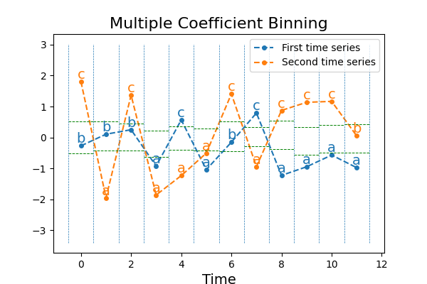
Multiple Coefficient Binning

Binning continuous data into intervals can be seen as an approximation that reduces noise and captures the trend of a time series. The Multiple Coefficient Binning (MCB) algorithm bins continuous time series into intervals, transforming each time point of all the time series (a sequence of floats) into a sequence of symbols, usually letters. Contrary to SAX which bins each time series independently, MCB bins each time point independently. This example shows how to use this algorithm and illustrates the transformation. It is implemented as pyts.approximation.MultipleCoefficientBinning.

# Author: Johann Faouzi <johann.faouzi@gmail.com>
# License: BSD-3-Clause

import numpy as np
import matplotlib.pyplot as plt
from pyts.approximation import MultipleCoefficientBinning

# Parameters
n_samples, n_timestamps = 100, 12

# Toy dataset
rng = np.random.RandomState(41)
X = rng.randn(n_samples, n_timestamps)

# MCB transformation
n_bins = 3
mcb = MultipleCoefficientBinning(n_bins=n_bins, strategy='quantile')
X_mcb = mcb.fit_transform(X)

# Show the results for two time series
plt.figure(figsize=(6, 4))

plt.plot(X[0], 'o--', ms=4, label='First time series')
for x, y, s in zip(range(n_timestamps), X[0], X_mcb[0]):
    plt.text(x, y, s, ha='center', va='bottom', fontsize=14, color='C0')

plt.plot(X[5], 'o--', ms=4, label='Second time series')
for x, y, s in zip(range(n_timestamps), X[5], X_mcb[5]):
    plt.text(x, y, s, ha='center', va='bottom', fontsize=14, color='C1')

# Plot the bin edges
for i in range(n_bins - 1):
    plt.hlines(mcb.bin_edges_.T[i], np.arange(n_timestamps) - 0.5,
               np.arange(n_timestamps) + 0.5, color='g',
               linestyles='--', linewidth=0.7)
plt.vlines(np.arange(n_timestamps + 1) - 0.5, X.min(), X.max(),
           linestyles='--', linewidth=0.5)

plt.legend(loc='best', fontsize=10)
plt.xlabel('Time', fontsize=14)
plt.title("Multiple Coefficient Binning", fontsize=16)
plt.show()