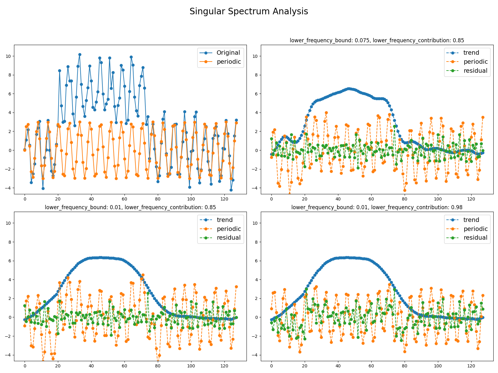
Trend-Seasonal decomposition with Singular Spectrum Analysis

Time series can be composed of three different subseries: trend, seasonal and noise. Decomposing time series into these components can be useful in order to characterize the underlying signal. One decomposition algorithm is Singular Spectrum Analysis. This example illustrates the decomposition of a time series into the three subseries using the automatic grouping of the SSA-components and visualizes the results depending on the selected parameters. It is implemented as pyts.decomposition.SingularSpectrumAnalysis.

# Author: Lucas Plagwitz <lucas.plagwitz@uni-muenster.de>
# License: BSD-3-Clause

import numpy as np
import matplotlib.pyplot as plt
from pyts.decomposition import SingularSpectrumAnalysis
from pyts.datasets import make_cylinder_bell_funnel

# Parameters
n_samples, n_timestamps = 3, 128

X_cbf, y = make_cylinder_bell_funnel(n_samples=10, random_state=42,
                                     shuffle=False)
X_period = 3 * np.sin(np.arange(n_timestamps))

X = X_cbf[:, :n_timestamps] + X_period

# We decompose the time series into three subseries
window_size = 20
# Singular Spectrum Analysis
ssa = SingularSpectrumAnalysis(window_size=window_size, groups="auto")
X_ssa = ssa.fit_transform(X)

# Show the results for different frequency-parameters
plt.figure(figsize=(16, 12))

ax1 = plt.subplot(221)
ax1.plot(X[0], 'o-', label='Original')
ax1.plot(X_period, 'o-', label='periodic')
ax1.legend(loc='best', fontsize=14)
ax1.set_ylim([np.min(X[0])*1.1, np.max(X[0])*1.1])

params = [(0.01, 0.85), (0.01, 0.98)]

for idx in range(3):
    ax = plt.subplot(222 + idx)
    labels = ["trend", "periodic", "residual"]
    for i in range(3):
        ax.plot(X_ssa[0, i], 'o--', label=labels[i])
    ax.legend(loc='best', fontsize=14)
    ax.set_ylim([np.min(X[0])*1.1, np.max(X[0])*1.1])
    ax.set_title(f"lower_frequency_bound: {ssa.lower_frequency_bound}, "
                 f"lower_frequency_contribution: "
                 f"{ssa.lower_frequency_contribution}")

    if idx > 1:
        continue
    ssa = SingularSpectrumAnalysis(window_size=window_size, groups="auto",
                                   lower_frequency_bound=params[idx][0],
                                   lower_frequency_contribution=params[idx][1])
    X_ssa = ssa.fit_transform(X)

plt.suptitle('Singular Spectrum Analysis', fontsize=20)

plt.tight_layout()
plt.subplots_adjust(top=0.88)
plt.show()