Transformers

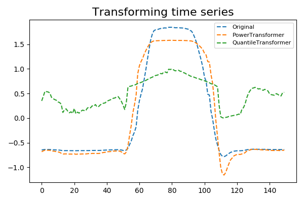
Some algorithms make assumptions on the distribution of the data. Therefore it can be useful to transform time series so that they approximatively follow a given distribution. Two transformers are made available:

• pyts.preprocessing.PowerTransformer
• pyts.preprocessing.QuantileTransformer.

This example illustrates the transformation from both algorithms.

# Author: Johann Faouzi <johann.faouzi@gmail.com>
# License: BSD-3-Clause

import matplotlib.pyplot as plt
from pyts.datasets import load_gunpoint
from pyts.preprocessing import PowerTransformer, QuantileTransformer

X, _, _, _ = load_gunpoint(return_X_y=True)
n_timestamps = X.shape[1]

# Transform the data with different transformation algorithms
X_power = PowerTransformer().transform(X)
X_quantile = QuantileTransformer(n_quantiles=n_timestamps).transform(X)

# Show the results for the first time series
plt.figure(figsize=(6, 4))
plt.plot(X[0], '--', label='Original')
plt.plot(X_power[0], '--', label='PowerTransformer')
plt.plot(X_quantile[0], '--', label='QuantileTransformer')
plt.legend(loc='best', fontsize=8)
plt.title('Transforming time series', fontsize=16)
plt.tight_layout()
plt.show()