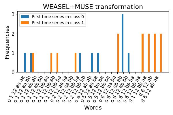
WEASEL+MUSE

WEASELMUSE stand for Word ExtrAction for time SEries cLassification plus Multivariate Unsupervised Symbols and dErivatives. This example shows how the WEASELMUSE algorithm transforms multivariate time series of real numbers into a sequence of frequencies of words, and illustrates the features obtained for two time series. It is implemented as pyts.multivariate.transformation.WEASELMUSE.

# Author: Johann Faouzi <johann.faouzi@gmail.com>
# License: BSD-3-Clause

import numpy as np
import matplotlib.pyplot as plt
from pyts.datasets import load_basic_motions
from pyts.multivariate.transformation import WEASELMUSE
from sklearn.preprocessing import LabelEncoder

# Toy dataset
X_train, _, y_train, _ = load_basic_motions(return_X_y=True)
y_train = LabelEncoder().fit_transform(y_train)

# WEASEL+MUSE transformation
transformer = WEASELMUSE(word_size=2, n_bins=2, window_sizes=[12, 36],
                         chi2_threshold=15, sparse=False)
X_weasel = transformer.fit_transform(X_train, y_train)

# Visualize the transformation for the first time series
plt.figure(figsize=(6, 4))
vocabulary_length = len(transformer.vocabulary_)
width = 0.3
plt.bar(np.arange(vocabulary_length) - width / 2, X_weasel[y_train == 0][0],
        width=width, label='First time series in class 0')
plt.bar(np.arange(vocabulary_length) + width / 2, X_weasel[y_train == 1][0],
        width=width, label='First time series in class 1')
plt.xticks(np.arange(vocabulary_length),
           np.vectorize(transformer.vocabulary_.get)(
               np.arange(X_weasel[0].size)),
           fontsize=12, rotation=60, ha='right')
y_max = np.max(np.concatenate([X_weasel[y_train == 0][0],
                               X_weasel[y_train == 1][0]]))
plt.yticks(np.arange(y_max + 1), fontsize=12)
plt.xlabel("Words", fontsize=14)
plt.ylabel("Frequencies", fontsize=14)
plt.title("WEASEL+MUSE transformation", fontsize=16)
plt.legend(loc='best', fontsize=10)

plt.subplots_adjust(bottom=0.27)
plt.tight_layout()
plt.show()