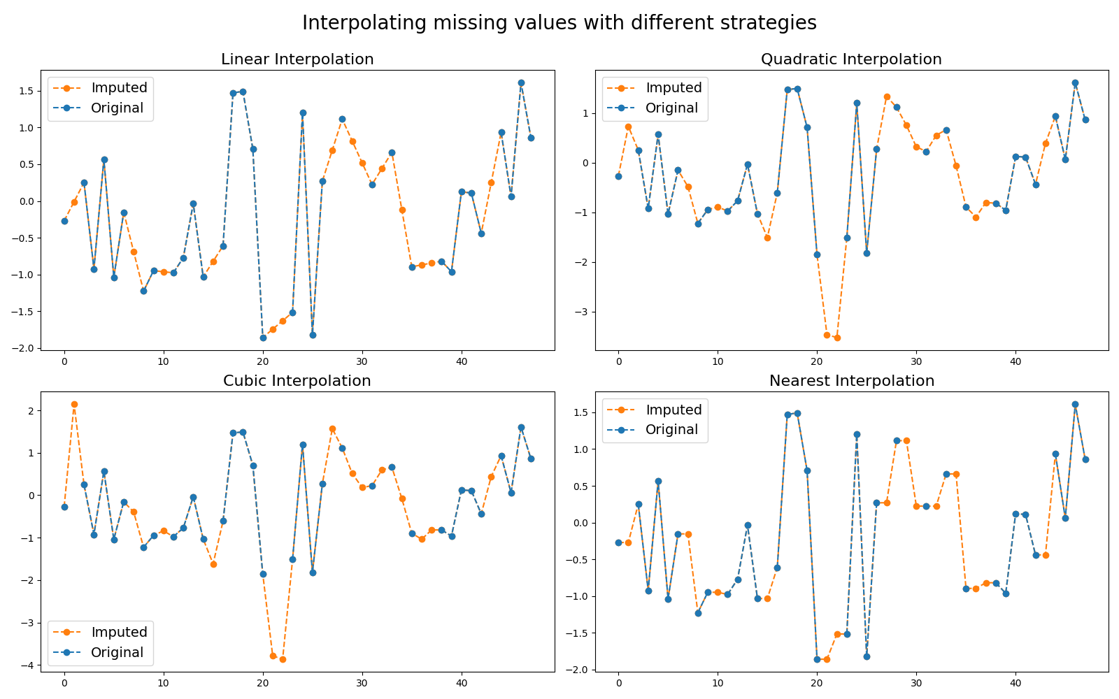
Imputer

Missing values are common in real-word datasets and most algorithms cannot deal with them. Thus it is standard to impute them. For time series, the imputation is based on interpolation from other time points in order to preserve temporal correlation between consecutive time points. Different strategies for interpolation are made available. This example illustrates these different strategies. It is implemented as pyts.preprocessing.InterpolationImputer.

# Author: Johann Faouzi <johann.faouzi@gmail.com>
# License: BSD-3-Clause

import numpy as np
import matplotlib.pyplot as plt
from pyts.preprocessing import InterpolationImputer

# Parameters
n_samples, n_timestamps = 100, 48

# Toy dataset
rng = np.random.RandomState(41)
X = rng.randn(n_samples, n_timestamps)
missing_idx = rng.choice(np.arange(1, 47), size=14, replace=False)
X[:, missing_idx] = np.nan

# Show the results for different strategies for the first time series
plt.figure(figsize=(16, 10))
for i, strategy in enumerate(['linear', 'quadratic', 'cubic', 'nearest']):
    imputer = InterpolationImputer(strategy=strategy)
    X_imputed = imputer.transform(X)

    plt.subplot(2, 2, i + 1)
    plt.plot(X_imputed[0], 'o--', color='C1', label='Imputed')
    plt.plot(X[0], 'o--', color='C0', label='Original')
    plt.title("{0} Interpolation".format(strategy.capitalize()), fontsize=16)
    plt.legend(loc='best', fontsize=14)

plt.suptitle('Interpolating missing values with different strategies',
             fontsize=20)
plt.tight_layout()
plt.subplots_adjust(top=0.9)
plt.show()