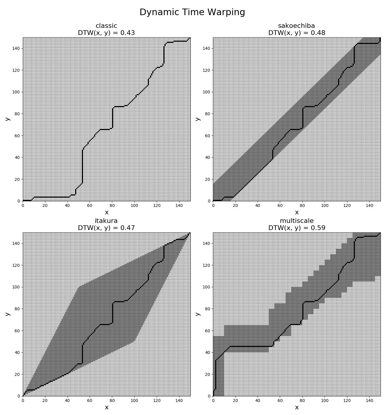
Dynamic Time Warping

This example shows how to compute and visualize the optimal path when computing Dynamic Time Warping (DTW) between two time series and compare the results with different variants of DTW. It is implemented as pyts.metrics.dtw().

import numpy as np
import matplotlib.pyplot as plt
from pyts.datasets import load_gunpoint
from pyts.metrics import dtw, itakura_parallelogram, sakoe_chiba_band
from pyts.metrics.dtw import (cost_matrix, accumulated_cost_matrix,
                              _return_path, _multiscale_region)

# Parameters
X, _, _, _ = load_gunpoint(return_X_y=True)
x, y = X[0], X[1]
n_timestamps = x.size

plt.figure(figsize=(13, 14))
timestamps = np.arange(n_timestamps + 1)

# Dynamic Time Warping: classic
dtw_classic, path_classic = dtw(x, y, dist='square',
                                method='classic', return_path=True)
matrix_classic = np.zeros((n_timestamps + 1, n_timestamps + 1))
matrix_classic[tuple(path_classic)[::-1]] = 1.

plt.subplot(2, 2, 1)
plt.pcolor(timestamps, timestamps, matrix_classic,
           edgecolors='k', cmap='Greys')
plt.xlabel('x', fontsize=16)
plt.ylabel('y', fontsize=16)
plt.title("{0}\nDTW(x, y) = {1:.2f}".format('classic', dtw_classic),
          fontsize=16)

# Dynamic Time Warping: sakoechiba
window_size = 0.1
dtw_sakoechiba, path_sakoechiba = dtw(
    x, y, dist='square', method='sakoechiba',
    options={'window_size': window_size}, return_path=True
)
band = sakoe_chiba_band(n_timestamps, window_size=window_size)
matrix_sakoechiba = np.zeros((n_timestamps + 1, n_timestamps + 1))
for i in range(n_timestamps):
    matrix_sakoechiba[i, np.arange(*band[:, i])] = 0.5
matrix_sakoechiba[tuple(path_sakoechiba)[::-1]] = 1.

plt.subplot(2, 2, 2)
plt.pcolor(timestamps, timestamps, matrix_sakoechiba,
           edgecolors='k', cmap='Greys')
plt.xlabel('x', fontsize=16)
plt.ylabel('y', fontsize=16)
plt.title("{0}\nDTW(x, y) = {1:.2f}".format('sakoechiba', dtw_sakoechiba),
          fontsize=16)

# Dynamic Time Warping: itakura
dtw_itakura, path_itakura = dtw(
    x, y, dist='square', method='itakura',
    options={'max_slope': 2.}, return_path=True
)
parallelogram = itakura_parallelogram(n_timestamps, max_slope=2.)
matrix_itakura = np.zeros((n_timestamps + 1, n_timestamps + 1))
for i in range(n_timestamps):
    matrix_itakura[i, np.arange(*parallelogram[:, i])] = 0.5
matrix_itakura[tuple(path_itakura)[::-1]] = 1.

plt.subplot(2, 2, 3)
plt.pcolor(timestamps, timestamps, matrix_itakura,
           edgecolors='k', cmap='Greys')
plt.xlabel('x', fontsize=16)
plt.ylabel('y', fontsize=16)
plt.title("{0}\nDTW(x, y) = {1:.2f}".format('itakura', dtw_itakura),
          fontsize=16)

# Dynamic Time Warping: multiscale
resolution, radius = 5, 4
dtw_multiscale, path_multiscale = dtw(
    x, y, dist='square', method='multiscale',
    options={'resolution': resolution, 'radius': radius}, return_path=True
)
x_padded = x.reshape(-1, resolution).mean(axis=1)
y_padded = y.reshape(-1, resolution).mean(axis=1)
cost_mat_res = cost_matrix(x_padded, y_padded, dist='square', region=None)
acc_cost_mat_res = accumulated_cost_matrix(cost_mat_res)
path_res = _return_path(acc_cost_mat_res)
multiscale_region = _multiscale_region(
    n_timestamps, resolution, x_padded.size, path_res, radius=radius
)
matrix_multiscale = np.zeros((n_timestamps + 1, n_timestamps + 1))
for i in range(n_timestamps):
    matrix_multiscale[i, np.arange(*multiscale_region[:, i])] = 0.5
matrix_multiscale[tuple(path_multiscale)[::-1]] = 1.

plt.subplot(2, 2, 4)
plt.pcolor(timestamps, timestamps, matrix_multiscale,
           edgecolors='k', cmap='Greys')
plt.xlabel('x', fontsize=16)
plt.ylabel('y', fontsize=16)
plt.title("{0}\nDTW(x, y) = {1:.2f}".format('multiscale', dtw_multiscale),
          fontsize=16)

plt.suptitle("Dynamic Time Warping", fontsize=22)
plt.tight_layout()
plt.subplots_adjust(top=0.91)
plt.show()