Note
Click here to download the full example code
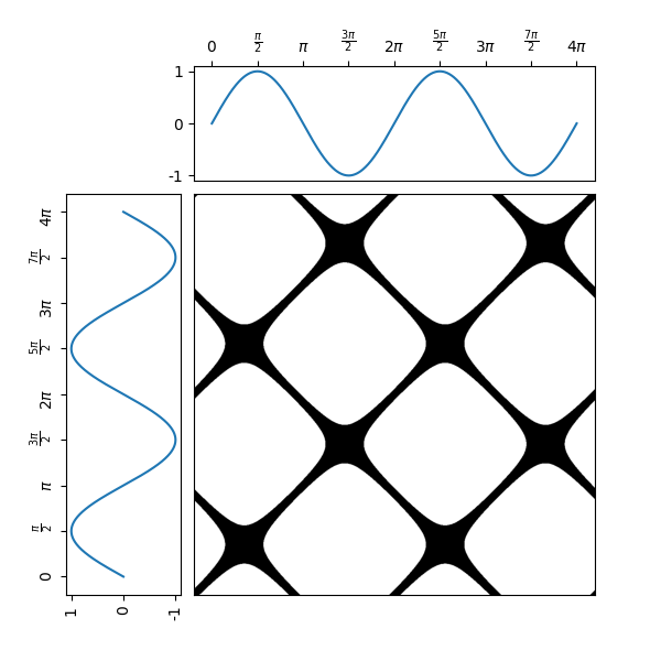
Single recurrence plot
A recurrence plot is an image obtained from a time series, representing the
pairwise Euclidean distances for each value (and more generally for each
trajectory) in the time series.
The image can be binarized using a threshold.
It is implemented as pyts.image.RecurrencePlot.
In this example, the considered time series is the sequence of the sine
function values for 1000 equally-spaced points in the interval
![[0, 4\pi]](../../_images/math/7945331ff3f9126f3967ca0ddc2185481f24eb33.svg) and the threshold used is 0.1.
One can see on the recurrence plot that the sine function is periodic with
period
and the threshold used is 0.1.
One can see on the recurrence plot that the sine function is periodic with
period  and that its derivative take lower absolute values around
 for any integer
  (because of the higher
density of black pixels).
(because of the higher
density of black pixels).
Since the API is designed for machine learning, the
transform() method of the
pyts.image.RecurrencePlot class expects a data set of time series
as input, so the time series is transformed into a data set with a single time
series (X = np.array([x])) and the first element of the data set of
recurrence plots is retrieved (ax_rp.imshow(X_rp[0], ...).
# Author: Johann Faouzi <johann.faouzi@gmail.com>
# License: BSD-3-Clause

import numpy as np
import matplotlib.pyplot as plt
from pyts.image import RecurrencePlot


# Create a toy time series using the sine function
time_points = np.linspace(0, 4 * np.pi, 1000)
x = np.sin(time_points)
X = np.array([x])

# Recurrence plot transformation
rp = RecurrencePlot(threshold=np.pi/18)
X_rp = rp.transform(X)

# Plot the time series and its recurrence plot
fig = plt.figure(figsize=(6, 6))

gs = fig.add_gridspec(2, 2,  width_ratios=(2, 7), height_ratios=(2, 7),
                      left=0.1, right=0.9, bottom=0.1, top=0.9,
                      wspace=0.05, hspace=0.05)

# Define the ticks and their labels for both axes
time_ticks = np.linspace(0, 4 * np.pi, 9)
time_ticklabels = [r'$0$', r'$\frac{\pi}{2}$', r'$\pi$',
                   r'$\frac{3\pi}{2}$', r'$2\pi$', r'$\frac{5\pi}{2}$',
                   r'$3\pi$', r'$\frac{7\pi}{2}$', r'$4\pi$']
value_ticks = [-1, 0, 1]
reversed_value_ticks = value_ticks[::-1]

# Plot the time series on the left with inverted axes
ax_left = fig.add_subplot(gs[1, 0])
ax_left.plot(x, time_points)
ax_left.set_xticks(reversed_value_ticks)
ax_left.set_xticklabels(reversed_value_ticks, rotation=90)
ax_left.set_yticks(time_ticks)
ax_left.set_yticklabels(time_ticklabels, rotation=90)
ax_left.invert_xaxis()

# Plot the time series on the top
ax_top = fig.add_subplot(gs[0, 1])
ax_top.plot(time_points, x)
ax_top.set_xticks(time_ticks)
ax_top.set_xticklabels(time_ticklabels)
ax_top.set_yticks(value_ticks)
ax_top.set_yticklabels(value_ticks)
ax_top.xaxis.tick_top()

# Plot the recurrence plot on the bottom right
ax_rp = fig.add_subplot(gs[1, 1])
ax_rp.imshow(X_rp[0], cmap='binary', origin='lower',
             extent=[0, 4 * np.pi, 0, 4 * np.pi])
ax_rp.set_xticks([])
ax_rp.set_yticks([])

plt.show()
Total running time of the script: ( 0 minutes 0.284 seconds)
