Note
Click here to download the full example code
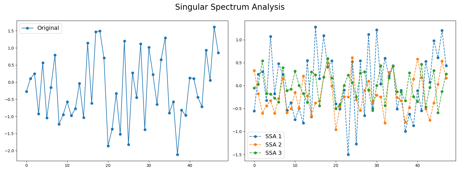
Singular Spectrum Analysis
Signals such as time series can be seen as a sum of different signals such
as trends and noise. Decomposing time series into several time series can
be useful in order to keep the most important information. One decomposition
algorithm is Singular Spectrum Analysis. This example illustrates the
decomposition of a time series into several subseries using this algorithm and
visualizes the different subseries extracted.
It is implemented as pyts.decomposition.SingularSpectrumAnalysis.
# Author: Johann Faouzi <johann.faouzi@gmail.com>
# License: BSD-3-Clause

import numpy as np
import matplotlib.pyplot as plt
from pyts.decomposition import SingularSpectrumAnalysis

# Parameters
n_samples, n_timestamps = 100, 48

# Toy dataset
rng = np.random.RandomState(41)
X = rng.randn(n_samples, n_timestamps)

# We decompose the time series into three subseries
window_size = 15
groups = [np.arange(i, i + 5) for i in range(0, 11, 5)]

# Singular Spectrum Analysis
ssa = SingularSpectrumAnalysis(window_size=15, groups=groups)
X_ssa = ssa.fit_transform(X)

# Show the results for the first time series and its subseries
plt.figure(figsize=(16, 6))

ax1 = plt.subplot(121)
ax1.plot(X[0], 'o-', label='Original')
ax1.legend(loc='best', fontsize=14)

ax2 = plt.subplot(122)
for i in range(len(groups)):
    ax2.plot(X_ssa[0, i], 'o--', label='SSA {0}'.format(i + 1))
ax2.legend(loc='best', fontsize=14)

plt.suptitle('Singular Spectrum Analysis', fontsize=20)

plt.tight_layout()
plt.subplots_adjust(top=0.88)
plt.show()

# The first subseries consists of the trend of the original time series.
# The second and third subseries consist of noise.
Total running time of the script: ( 0 minutes 3.365 seconds)
