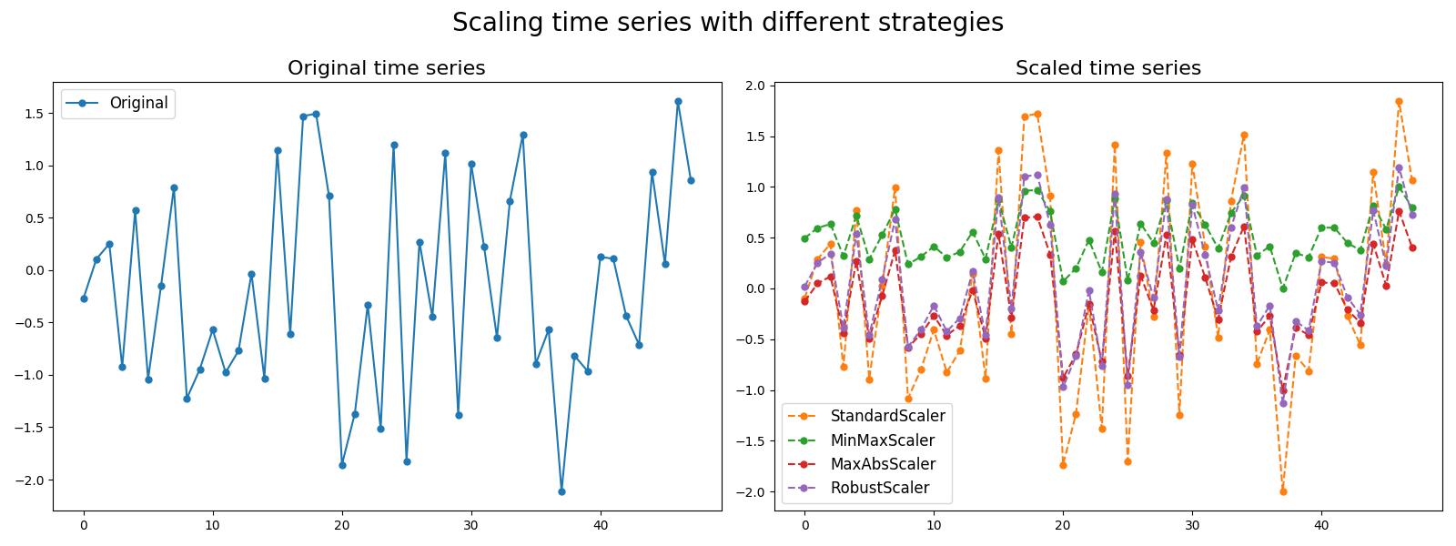
Scalers

This example shows the different scaling algorithms available in pyts.preprocessing.

import numpy as np
import matplotlib.pyplot as plt
from pyts.preprocessing import (StandardScaler, MinMaxScaler,
                                MaxAbsScaler, RobustScaler)

# Parameters
n_samples, n_timestamps = 100, 48
marker_size = 5

# Toy dataset
rng = np.random.RandomState(41)
X = rng.randn(n_samples, n_timestamps)

# Scale the data with different scaling algorithms
X_standard = StandardScaler().transform(X)
X_minmax = MinMaxScaler(sample_range=(0, 1)).transform(X)
X_maxabs = MaxAbsScaler().transform(X)
X_robust = RobustScaler(quantile_range=(25.0, 75.0)).transform(X)

# Show the results for the first time series
plt.figure(figsize=(16, 6))

ax1 = plt.subplot(121)
ax1.plot(X[0], 'o-', ms=marker_size, label='Original')
ax1.set_title('Original time series', fontsize=16)
ax1.legend(loc='best', fontsize=12)

ax2 = plt.subplot(122)
ax2.plot(X_standard[0], 'o--', ms=marker_size, color='C1',
         label='StandardScaler')
ax2.plot(X_minmax[0], 'o--', ms=marker_size, color='C2', label='MinMaxScaler')
ax2.plot(X_maxabs[0], 'o--', ms=marker_size, color='C3', label='MaxAbsScaler')
ax2.plot(X_robust[0], 'o--', ms=marker_size, color='C4', label='RobustScaler')
ax2.set_title('Scaled time series', fontsize=16)
ax2.legend(loc='best', fontsize=12)

plt.suptitle('Scaling time series with different strategies', fontsize=20)
plt.tight_layout()
plt.subplots_adjust(top=0.85)
plt.show()