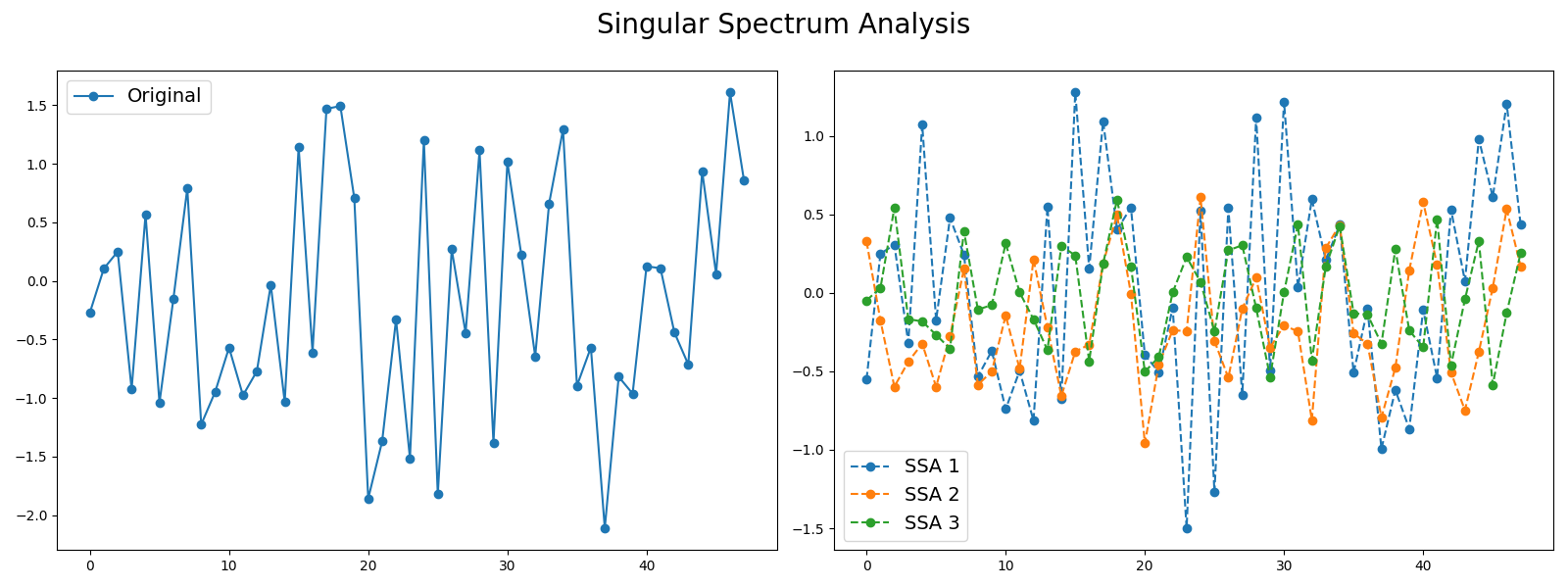
Singular Spectrum Analysis

This example shows how you can decompose a time series into several time series using pyts.decomposition.SingularSpectrumAnalysis.

import numpy as np
import matplotlib.pyplot as plt
from pyts.decomposition import SingularSpectrumAnalysis

# Parameters
n_samples, n_timestamps = 100, 48

# Toy dataset
rng = np.random.RandomState(41)
X = rng.randn(n_samples, n_timestamps)

# We decompose the time series into three subseries
window_size = 15
groups = [np.arange(i, i + 5) for i in range(0, 11, 5)]

# Singular Spectrum Analysis
ssa = SingularSpectrumAnalysis(window_size=15, groups=groups)
X_ssa = ssa.fit_transform(X)

# Show the results for the first time series and its subseries
plt.figure(figsize=(16, 6))

ax1 = plt.subplot(121)
ax1.plot(X[0], 'o-', label='Original')
ax1.legend(loc='best', fontsize=14)

ax2 = plt.subplot(122)
for i in range(len(groups)):
    ax2.plot(X_ssa[0, i], 'o--', label='SSA {0}'.format(i + 1))
ax2.legend(loc='best', fontsize=14)

plt.suptitle('Singular Spectrum Analysis', fontsize=20)

plt.tight_layout()
plt.subplots_adjust(top=0.88)
plt.show()

# The first subseries consists of the trend of the original time series.
# The second and third subseries consist of noise.