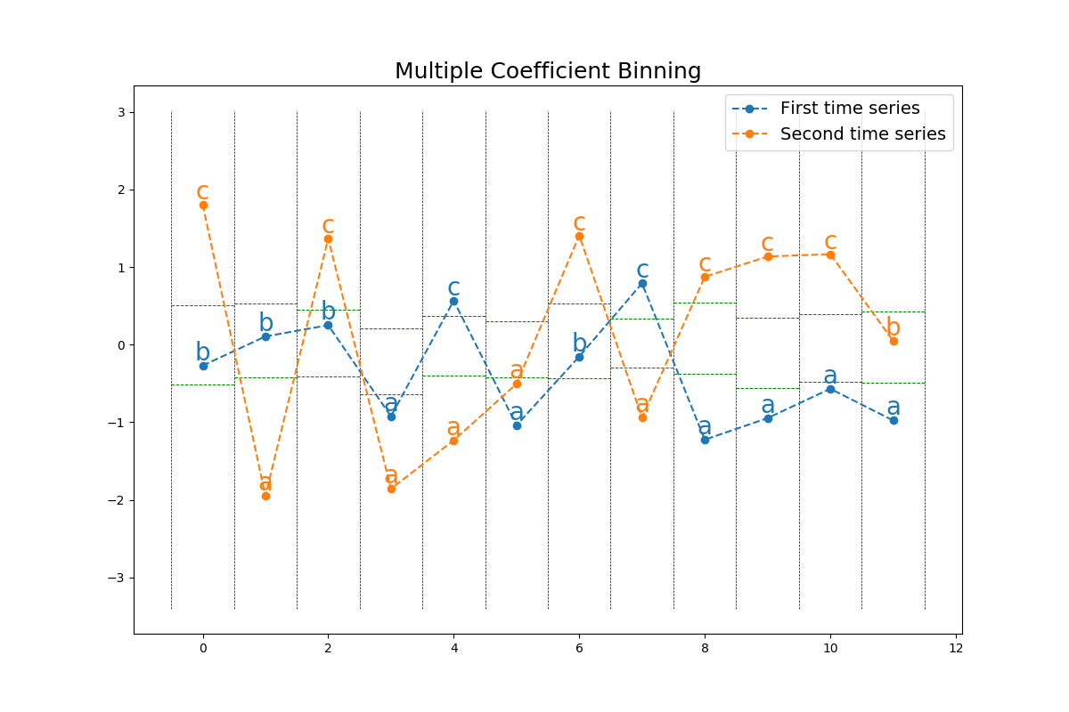
Multiple Coefficient Binning

This example shows how the Multiple Coefficient Binning algorithm transforms a dataset of time series of real numbers into a list of sequences of symbols. It is implemented as pyts.approximation.MultipleCoefficientBinning.

import numpy as np
import matplotlib.pyplot as plt
from pyts.approximation import MultipleCoefficientBinning

# Parameters
n_samples, n_timestamps = 100, 12

# Toy dataset
rng = np.random.RandomState(41)
X = rng.randn(n_samples, n_timestamps)

# MCB transformation
n_bins = 3
mcb = MultipleCoefficientBinning(n_bins=n_bins, strategy='quantile')
X_mcb = mcb.fit_transform(X)

# Show the results for two time series
plt.figure(figsize=(12, 8))

plt.plot(X[0], 'o--', label='First time series')
for x, y, s in zip(range(n_timestamps), X[0], X_mcb[0]):
    plt.text(x, y, s, ha='center', va='bottom', fontsize=20, color='C0')

plt.plot(X[5], 'o--', label='Second time series')
for x, y, s in zip(range(n_timestamps), X[5], X_mcb[5]):
    plt.text(x, y, s, ha='center', va='bottom', fontsize=20, color='C1')

plt.hlines(mcb.bin_edges_.T, np.arange(n_timestamps) - 0.5,
           np.arange(n_timestamps) + 0.5, color='g',
           linestyles='--', linewidth=0.7)
plt.vlines(np.arange(n_timestamps + 1) - 0.5, X.min(), X.max(),
           linestyles='--', linewidth=0.5)

plt.legend(loc='best', fontsize=14)
plt.title("Multiple Coefficient Binning", fontsize=18)
plt.show()