Note
Click here to download the full example code
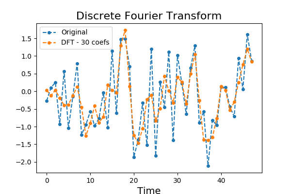
Discrete Fourier Transform
Discrete Fourier Transform is a signal processing technique that transforms
a signal of size n into a vector of complex Fourier coefficients of size n.
When the signal consists of floats, the transformation can be made bijective
and consists of a vector of floats of size n. The first Fourier coefficients
are the coefficients from the lowest frequencies and represent the trend,
while the last Fourier coefficients are for the highest frequencies and
usually represent noise. A time series can thus be approximated using some
of the first Fourier coefficients. This example illustrates the difference
between the original time series and the time series approximated with the
first Fourier coefficients.
It is implemented as pyts.approximation.DiscreteFourierTransform.
# Author: Johann Faouzi <johann.faouzi@gmail.com>
# License: BSD-3-Clause

import numpy as np
import matplotlib.pyplot as plt
from pyts.approximation import DiscreteFourierTransform

# Parameters
n_samples, n_timestamps = 100, 48

# Toy dataset
rng = np.random.RandomState(41)
X = rng.randn(n_samples, n_timestamps)

# DFT transformation
n_coefs = 30
dft = DiscreteFourierTransform(n_coefs=n_coefs, norm_mean=False,
                               norm_std=False)
X_dft = dft.fit_transform(X)

# Compute the inverse transformation
if n_coefs % 2 == 0:
    real_idx = np.arange(1, n_coefs, 2)
    imag_idx = np.arange(2, n_coefs, 2)
    X_dft_new = np.c_[
        X_dft[:, :1],
        X_dft[:, real_idx] + 1j * np.c_[X_dft[:, imag_idx],
                                        np.zeros((n_samples, ))]
    ]
else:
    real_idx = np.arange(1, n_coefs, 2)
    imag_idx = np.arange(2, n_coefs + 1, 2)
    X_dft_new = np.c_[
        X_dft[:, :1],
        X_dft[:, real_idx] + 1j * X_dft[:, imag_idx]
    ]
X_irfft = np.fft.irfft(X_dft_new, n_timestamps)

# Show the results for the first time series
plt.figure(figsize=(6, 4))
plt.plot(X[0], 'o--', ms=4, label='Original')
plt.plot(X_irfft[0], 'o--', ms=4, label='DFT - {0} coefs'.format(n_coefs))
plt.legend(loc='best', fontsize=10)
plt.xlabel('Time', fontsize=14)
plt.title('Discrete Fourier Transform', fontsize=16)
plt.show()
Total running time of the script: ( 0 minutes 0.126 seconds)
